Scan Model & Likelihood Fields

COMP329 Lectures 2022-10-20

Refer to the slides, from 81-94 for this lecture as there are a lot of diagrams.

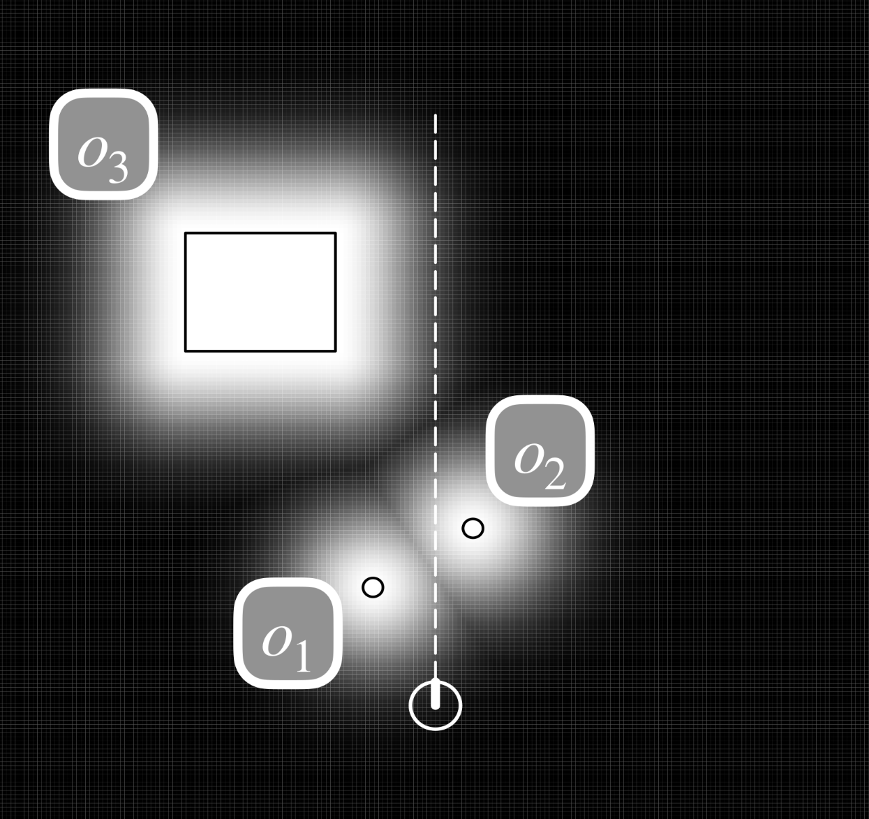
Consider we have a map with objects in it. We can make a likelihood field by applying a Gaussian distribution to the edge of each object in the map.

Modelling a Robot with 6 Sensors

• There is a worked example in the slides of calculating the pose of each sensor on a robot.

Finding the Location of Scan $z_t$

To find the location of a scan $z_t$ in global coordinate space:

• Let robot pose at time $t$ be $x_t=\langle x,y,\theta\rangle$.
• Relative to the robot coordinate space, sensor $\text{sens}_k$ has:
  • Location $\langle x_{k,\text{sens}}, y_{k,\text{sens}}\rangle$.
  • Rotation $\theta_{k,\text{sens}}$ relative to the pose of the robot.
• Let $z^k_t$ be the end point of a measurement from sensor $\text{sens}_k$.

• The location of $z_t^k$ is given at $(x_{z_t^k}, x_{z_t^k})^T$ where:

  \[\begin{pmatrix}x_{z_t^k}\\y_{z_t^k}\end{pmatrix}= \underbrace{\begin{pmatrix}x\\y\end{pmatrix}}_\text{Robot Location}+ \underbrace{\begin{pmatrix}\cos\theta&-\sin\theta\\\sin\theta&\cos\theta\end{pmatrix} \begin{pmatrix}x_{k,\text{sens}}\\y_{k,\text{sens}}\end{pmatrix}}_{\substack{\text{The location of the sensor (relative to the}\\\text{ robot) rotated by the robot's heading}}}+ \underbrace{z_t^k\begin{pmatrix}\cos(\theta+\theta_{k,\text{sens}})\\\sin(\theta+\theta_{k,\text{sens}})\end{pmatrix}}_{\substack{\text{The combined robot's heading and sensor}\\\text{orientation scaled with the measured range}}}\]

Calculating the Likelihood Field

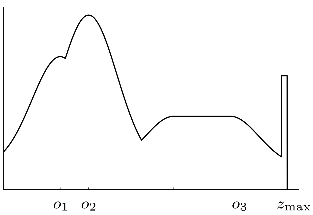
As with the beam model we combine the weighted sum of the three distributions:

For scan models, we omit unexpected obstacles.

• Measurement Noise

  \[P_\text{hit}=\eta\frac1{\sqrt{2\pi b}}e^{-\frac12\frac{(z-z_\text{exp})^2}{b}}\]

• Random Measurements

  \[P_\text{rand}=(z\mid x, m) = \begin{cases} \frac1{z_\max}&\text{if }0\leq z\leq z_\max\\ 0&\text{otherwise} \end{cases}\]

• Max Range

  \[P_\text{max}=\begin{cases}1&z=z_\max\\0&\text{otherwise}\end{cases}\]

We can combine this by calculating the weighted sum of all the distributions:

\[P(z\mid x, m)=\begin{pmatrix} \alpha_\text{hit}\\ \alpha_\max\\ \alpha_\text{rand} \end{pmatrix}^T\cdot \begin{pmatrix} P_\text{hit}(z\mid x, m)\\ P_\text{max}(z\mid x, m)\\ P_\text{rand}(z\mid x, m)\\ \end{pmatrix}\]

where:

\[\alpha_\text{hit}+ \alpha_\max+ \alpha_\text{rand}=1\]