Views of AI
Typical AI Application Areas
- Natural Language Processing
- Computer Vision
- Robotics
- Theorem Proving
- Speech Recognition
- Game Playing
- Sematic Web Search
- Diagnosis
What is AI
The goal of AI is to build machines that perform tasks that normally require human intelligence. This can also be construed as what is new in computing as the computers performing the task can be seen as intelligent.
AI is both science and engineering as it is:
- the science of understanding intelligent entities: developing theories/models which attempt to explain and predict the nature of such entities.
- the engineering of such entities.
Four Views of AI
- Systems that think like humans
- Systems that act like humans
- Systems that think rationally (think the correct way)
- Systems that act rationally (act optimal to achieve a goal)
Thinking Humanly vs Acting Humanly
Computer science is concerned with acting intelligently rather than simulating a brain like a cognitive scientist might want. An abstract of this is whether they act intelligently. This is because although an entity might not think intelligently it can appear intelligent by acting intelligently.
Turing Test 1950
A human should not be able to tell whether an entity is a human or a machine.
No system has yet passed the test. In addition, it is not always the most practical or foolproof as those who are the most successful rely on tricks.
Thinking and Acting Rationally
This is the focus on making systems that act how we think that they should act. To do this we can use techniques from logic and probability theory to create machines that can reason correctly.
- Acting Rationally - Acting in such a way to achieve one’s goals optimally and given one’s beliefs.
As a result of this view, we can use techniques from economics/game theory to investigate and create machines that act rationally.
History of AI
Combinatorial Explosion - Chess
For a simple game it is possible to write a program that will select the best possible move from all possible moves. However in chess there are an exponential number of moves after each move.
The fact that a program can find a solution in principle
does not mean that the program will be able to find it in practice.
Expert systems
- As general purpose brute force techniques don’t work we should use knowledge rich solutions.
- These are very specialised systems with vast amounts of knowledge about a tightly focused domain.
The main problems with expert systems are:
- The knowledge elicitation bottleneck
- Finding knowledge from experts is very time consuming and expensive
- Lack of trust in recommendations given by expert systems
- The main problem as you don’t know how the system has came to the solution.
Entities that are engineered in AI are known as agents.
An agent is anything that can be viewed as perceiving its environment through sensors and acting upon that environment through actuators.
PEAS
- Performance Measure
- The criteria by which we can measure the success of an agent’s behaviour.
- Environment
- The external environment that the agent inhabits.
- Actuators
- The means by which the agent acts within its environment.
- Sensors
- The means by which the agent senses its environment.
Ex. Vacuum Cleaner
- Performance measure
- Environment
- A vacuum cleaner located in one of two rooms, each possibly containing dirt
- Actuators
- Move left/right, suck up the dirt, do nothing
- Sensors
- In which room is the vacuum cleaner? Is there dirt in that room?
Task Environments
Fully Observable vs Partially Observable
A fully observable environment is one in which the agent can fully obtain complete, up-to-date info about the environment’s state. Generally games can be fully observable but most real-life situations are partially observable.
Partially observable environments require a memory to deduce what might happen based on the last gained information.
Deterministic vs Stochastic
Deterministic environments are where any action has a single guaranteed effect. Stochastic means that there is no certainty about the outcome given a certain input.
Episodic vs Sequential
Episodic environments are where the performance of an agent is dependent on a number of discrete episodes with no link between it’s performance in each episode. In sequential environments different episodes are linked.
In sequential environments decisions made now may affect the future and must be taken into account.
Static vs Dynamic
In a static environment everything will stay the same while the agent is deliberating. This is common in turn based games. For dynamic environments things will change while the agent is deliberating and actions are more urgent.
Discrete vs Continuous
In a discrete environment there are a fixed number of distinct states. In continuous environments there can be many states such that we consider them as infinite.
Intelligent agents are classified depending on how they map their precepts to their actions. They can be classed under:
- Simple reflex agents
- Select actions to execute based upon the current percept
- Don’t take the percept history into account.
- Very simple IFTTT actions.
- Very simple to implement but have limited intelligence.
- They have no memory.
graph TB
    A(Environment)--> |Sensors| B
    B[What the world is like now] --> C
    C[What action I should do now]--> |Actuators| A
    D[Condition-action rules]-->C
- Model-based reflex agents
- Maintain an internal state that depends upon the percept history - memory.
- Helps deal with partial observability.
- Knows how the world evolves and how its actions affect the world.
graph TB
    A(Environment)--> |Sensors| B
    B[What the world is like now] --> C
    C[What action I should do now]--> |Actuators| A
    D[Condition-action rules]-->C
    E-->B
    B.->E(State)
    F(How the world evolves)-->B
    G(What my actions do)-->B
- Goal-based agents
- Select appropriate actions to achieve desirable state of the environment.
- Knowledge of the current state does not automatically mean that the agent knows what to do.
- It will have to plan what to do over a long sequence of actions.
graph TB
    A(Environment)  --> |Sensors| B
    B[What the world is like now] --> H
    H[What it will be like if I do action A] --> C
    C[What action I should do now]--> |Actuators| A
    D[Condition-action rules]-->C
    B.->E(State)
    E-->B
    F(How the world evolves)-->B
    F --> H
    G(What my actions do)-->B
    G --> H
- Utility-based agents
- Make use of a utility function to compare the desirability of different states that result from actions.
- Many actions may satisfy the goal but which one is the most desirable?
- Utility function maps a state, or sequence of states, onto a number to give the degree of usefulness of the state to the agents.
- Agent maximises the value of its utility function.
graph TB
    A(Environment)--> |Sensors| B
    B[What the world is like now] --> H
    H[What it will be like if I do action A] --> I
    I[How happy I will be in such a state] --> C
    J(Utility)-->I
    C[What action I should do now]--> |Actuators| A
    D[Condition-action rules]-->C
    B.->E(State)
    E-->B
    F(How the world evolves)-->B
    F --> H
    G(What my actions do)-->B
    G --> H
- Learning agents
- Learning agents find ways of maximising their utility function based on previous experience
- The performance element is the same choice mechanism from the previous agents. This is now informed by the learning element.
- The performance standard informs the learning element how well it’s actions have worked.
graph TB
	A(Environment) --> |Sensors| B[Performance element]
	B --> |Actuators| A
	D[Performance standard] --> C[Critic]
	C --> |Feedback| L[Learning element]
	L --> |Changes| B
	B --> |Knowledge| L
	L --> |Learning Goals| P[Problem Generator]
	P --> B
BFS and DFS are blind search algorithms meaning we have no further information about the tree.
Solving Problems by Searching
Considering that there is a goal-based agent that want to bring about a state of affairs by completing some actions. These actions need to be ordered in order to reach the goal. We may also want to minimise time or fuel consumption. This is all part of the problem formulation.
- Describing the Goal
- Describing the Relevant State of the Environment
- Describing the Possible Actions
- Describing the Optimality Criterion
Once the problem has been formulated, looking for a sequence of actions that lead to a goal state and is optimal is called search.
S are the possible states or nodes in a graph. There can be:
- S$_\textrm{start}$ for the starting point.
- S$_\textrm{goal}$ for the goal states.
- A set of A actions that can be performed that will take the agent from one state in S to another state in S.
- There can sometimes be a cost function that states how expensive an action is. If all actions are equally expensive, we set $\textrm{cost}(a)=1$
A solution to the search problem is a sequence of actions such that when performed in the start state S$\textrm{start}$, that agents reaches a goal state in S$\textrm{goal}$. A solution is optimal if there is no less expensive solution.
Notation
For any node S, which is a state:
- The children are called successor states (s)
- The parents are called predecessor states (s’)
Abstraction
As the real world is very complex state space must be abstracted for problem solving. This can be seen as an abstract state could be any number of real states. In addition and abstract action could be any complex combination of real actions.
A good abstraction sound guarantee reasonability. E.g. Any one real state must get to another real state following the abstracted actions.
An abstract solution is a set of real paths that are solutions in the real world.
In real search problems the state space is huge e.g. Rubik’s Cube - $10^{18}$ which will take 68,000 years to brute force at 10 million states/sec. This is an example of the combinatorial explosion. In addition, we cannot store all of the states.
Instead, given the start state. We can describe the actions and compute the successor states. A description of the goal states can be given to check whether the goal is reached.
Search is the systematic exploration of the search tree consisting of all possible paths of states starting with the start state using the action available until a path to a goal state is reached.
Search Tree for Holiday in Romania
- Arad
- Arad, Sibiu and Arad, Timisoara and Arad, Zerind
Thus we have a Single path of length 0 and three paths of length 1. Later on going back is a valid path e.g. Arad, Sibiu, Arad.
The search algorithm says how to reach the nodes of the tree. Applying actions longer paths are generated by adding up successor states. This is called expanding the path/state.
graph TD
A[Arad] .-> S[Sibu]
A .-> T[Timisoara]
A .-> Z[Zerind]
S .-> A1[Arad]
S .-> Fagaras
S .-> Oradea
S .-> R[Rimnicu Vilcea]
T .-> A2[Arad]
T .-> Lugoj
Z .-> A3[Arad]
Z .-> O1[Oradea]
The initial state.
graph TD
A[Arad] --> S[Sibu]
A --> T[Timisoara]
A --> Z[Zerind]
S .-> A1[Arad]
S .-> Fagaras
S .-> Oradea
S .-> R[Rimnicu Vilcea]
T .-> A2[Arad]
T .-> Lugoj
Z .-> A3[Arad]
Z .-> O1[Oradea]
After expanding Arad.
graph TD
A[Arad] --> S[Sibu]
A --> T[Timisoara]
A --> Z[Zerind]
S --> A1[Arad]
S --> Fagaras
S --> Oradea
S --> R[Rimnicu Vilcea]
T .-> A2[Arad]
T .-> Lugoj
Z .-> A3[Arad]
Z .-> O1[Oradea]
After expanding Sibiu.
Input: 	a start state s_0
		for each state s the successors of s
		a test goals(s) checking whether s is a goal state

Set frontier := {s_0}
while frontier is not empty do
	select and remove from frontier a path s_0...s_k
	if goal(s_k) then
		return s_0...s_k (and terminate)
	else for every successor s of s_k and s_0...s_k s to frontier
	end if
end while
- Lines 1-3 are specifying the input of the program.
- Line 5 sets the frontier (the set of paths) to s$_0$.
- Line 7 remove a path and expand it.
- Lines 8-9 if the final state in the frontier is the goal state then return the path and end.
- Line 10 if the goal isn’t reached then add all expansions of successors to the frontier.
The algorithm maintains a set called the frontier containing the paths. It is also sometimes called the agenda. As long as the frontier is not empty is selects and removes a path from itself and adds the paths expansions. The differences between algorithms are with which path is removed and expanded in the frontier.
BFS vs DFS
In line 7, if you remove and expand the item that was added first that is called breadth first. If you remove and expand the one that was added last that is a depth first search.
Covering the tutorial sheets from week 1. The tutorial leader’s email is F.Alves@liverpool.ac.uk.
- The leader chose to cover one of the options which was football.
- Performance Measure
- Environment
- Football pitch, the players, the ball.
- Actuators
- Sensors
- Visual, hearing, pressure.
- Classification
- Partially observable environment as they can’t see what is behind them and they have to memorise the positions of the players that they can’t see.
- Stochastic as there is uncertainty about the state that will come from performing an action
- Sequential as the current decision could affect all future decisions.
- Dynamic environment as other players are acting while you make your decision.
- Continuous as there is no fixed states for the positions.
- Refer to the textbook or lecture notes.
- For a path $a_0 \rightarrow a_1 \rightarrow a_2 \rightarrow a_3$, the length of the path is 3 as that is the number of actions that need to be performed.
- When listing paths you can list them by length
- 0 : a
- 1 : ab, ac, ad
- 2 : abe, ace, ade
- 3 : abef, acef, adef
This may help with drawing search trees.
 graph LR
 a --> ab
 a --> ac
 a --> ad
 ab --> abe
 ac --> ace
 ad --> ade
 abe --> abef
 ace --> acef
 ade --> adef
-
- Paths
- 0 : a
- 1 : ab
- 2 : aba, abc
- 3 : abab
- 4 : ababa, ababc
- Search graph
graph LR
a --> ab
ab --> aba
ab --> abc
aba --> abab
abab --> ababa
abab --> ababc
ababc .-> A[ ]
You should draw the trailing arrow to indicate that the graph has bee truncated.
Search graphs should be drawn with the whole path at each level as it shows the full search at each level.
- Similar to 3. and 4.
-
- This problem is very large so I will describe the result
- The set of $S$ states are all 16 or $4^4$ states that exist as a subset of the set $N = \{ 1,2,3,4 \}$
- The start state $S_{start}$ is an empty subest $\{ \phi \}$ with a sum of zero.
- The set of goal states $S_{goal}$ are all the subsets which add to 6
- The set of actions $A$ are any addition or subtraction of a number that is in the set.
- The cost function for each action should just be one such that the shortest route from $S_{start}$ is achieved.
-
The search graph starts at level 1 with the empty list and then each subsequent level adds an additional item to the list via an action which adds or subtracts an item from the set:
  graph TD
  A[phi 0] --> |a1| B[<1> 1]
  A --> |+2| C[<2> 2]
  A --> |+3| D[<3> 3]
  A --> |+4| E[<4> 4]
  B --> |+2| F[<1,2> 3]
  B --> |+3| G[<1,3> 4]
  B --> |+4| H[<1,4> 5]
  C --> |+1| F
  C --> |+3| I[<2,3> 5]
  C --> |+4| J[<2,4> 6]
  D --> |+1| G
  D --> |+2| I
  D --> |+4| K[<3,4> 7]
  E --> |+1| H
  E --> |+2| J
  E --> |+3| K
  F .-> L[ ]
  G .-> M[ ]
  H .-> N[ ]
  I .-> O[ ]
  J .-> P[ ]
  K .-> Q[ ]
As you can see this is very tedious indeed.
- Select and expand start state to give a tree of depth 1.
- Select and expand all paths that resulted from previous step to give a tree of depth 2.
- and so on.
In general select adn expand all paths of depth $n$ before depth $n + 1$
Maze example
First explore paths of length 1, then depth 2 then length three. This has the result of following all paths and then returning to the source via the shortest path.
Example 1
graph TD
S --> A
S --> B
S --> C
A --> D
A --> E
B --> G
E --> G
C --> F
F --> G
D --> H
Example Graph.
| Expanded Paths |
Frontier |
| |
S |
| S not goal |
SA, SB, SC |
| SA not goal |
SB, SC, SAD, SAE |
| SB not goal |
SC, SAD, SAE, SBG |
| SC not goal |
SAD, SAE, SBG, SCF |
| SAD not goal |
SAE, SBG, SCF, SADH |
| SAE not goal |
SBG, SCF, SADH, SAEG |
| SBG is goal |
SCF, SADH, SAEG |
If the route was expanded at the same time then they are allowed to be added in any order. Otherwise they should be searched in the order that they were first added to the frontier. Choosing the first item in the frontier is always the right option as it is first in first out.
Depth first always selects the longest path from the frontier as opposed to the shortest path. From the perspective of the frontier you are expanding the path that was most recently added as opposed to the oldest path in the frontier.
Change to Pseudo-code
7:	select and remove from frontier the path s_o...s_k that was
8: 	last added to frontier
As a result a stack should be used instead of a queue such that the last into the data structure is the first out.
Example
graph TD
S --> A
S --> B
S --> C
A --> D
A --> E
B --> G
E --> G
C --> F
F --> G
D --> H
Example Graph.
| Expansion Paths |
Frontier |
| |
S |
| |
SA, SB, SC |
| SA is not goal |
SB, SC, SAD, SAE |
| SAD is not goal |
SB, SC, SAE, SADH |
| SADH is not goal |
SB, SC, SAE |
| SAE is not goal |
SB, SC, SAEG |
| SAEG is goal |
SB, SC |
This additionally illustrates that depth first doesn’t always find the shortest path as the longest paths are searched first.
Breadth first however always finds the shortest path.
For all algorithms there are certain properties that they can be evaluated against:
- Completeness
- Does the algorithm always find a solution if one exists?
This is true for BFS but not for DFS as cycles can stop depth first if there is a loop.
- Optimality
- Does the algorithm always find a shortest path or one of lowest cost?
Yes for BFS but no for DFS (neither take into account cost, just steps.)
- Time Complexity
- What are the number of paths generated?/How long will it take to compute?
Harder to answer. This will need to be computed
- Space Complexity
- What are the maximum number of paths in memory (in frontier)?
This will always be smaller or equal to the time complexity but it is still harder to answer.
Time & Space Complexity
Time and space complexity are measured in terms of:
- $b$ - Maximum branching factor
- The maximal number of successor states of a state in the state space.
- $d$ - Depth of the optimal solution
- The length of the shortest path from the start state to a goal state.
- $m$ - Maximum depth of the state space
- the length of the longest path in the state space (may be $\infty$ to to loops)
Example 1 - 8 Puzzle
- $b$ (maximum branching factor) is 4
- $d$ (optimal solution) is 31
- $m$ (longest path) is $\infty$ as there are cycles
Example 2 - Holiday in Romania
Properties of Breadth First Search
The number of paths of length $d$ in a search tree with maximum branching factor $b$ is at most $b^d$.
The number of paths of length at most $d$ in a search tree with maximum branching factor $b$ is at most $1+b+b^2+\ldots + b^d$.
- Time complexity
- If the shortest path to a goal state has length $d$ then the worst case BFS will look at: \(1+b+B^2+\ldots +b^d\) paths before reaching a goal state.
- Space complexity
- If the shortest path to a goal state has length $d$, then in the worst case the frontier can contain $b^d$ paths and so the memory requirement is $b^d$.
Complexity
| Depth |
Paths |
Time |
| 0 |
1 |
1 msec |
| 1 |
11 |
.01 sec |
| 2 |
111 |
.1 sec |
| 4 |
11,111 |
11 sec |
| 6 |
10^6 |
18 sec |
| 8 |
10^8 |
31 hours |
| 10 |
10^10 |
128 days |
| 12 |
10^12 |
35 years |
Example of combinatorial explosion of a BFS at 1000 states/sec.
Properties of Depth First Search
- Not complete - No guarenteed to find a solution
- Not optimal - Solution is not guaranteed to be the shortest path.
- Time Complexity
- If the length of the longest path from the start state is $m$, then the worst case DFS will look at: \(1+b+b^2+\ldots +b^m\) This may be an issue as $m$ is infinite in many problems.
- Space Complexity
- If the length of the longest path starting at a goal state is $m$, then the worst case the frontier can contain: \(b\times m\) paths. if $m$ is infinite, then the space requirement is infinite in the worst case. But if DFS finds a path to the goal state, then memory requirement is much less than for BFS.
Summary
- DFS is complete ut expensive
- DFS is cheap in space complexity but incomplete
Basic problem solving techniques such as BFS and DFS are either incomplete, in the case of DFS or computationally expensive.
You can make some tweaks to generate other uniform cost search algorithms or add more information to give an informed search algorithm. Either of these are an improvement
- Uniform cost search is similar to a BFS but including cost.
- Heuristic searches include rules of thumb and can include:
- Greedy search
- A* search
- This is the most easiest and most popular search method made in 1968.
Search Graph with Costs
A path cost function,
\(g:\text{Paths}\rightarrow\text{real numbers}\)
gives a cost to each path. We assume that the cost of a path is the sum over the costs of the steps in the path.
- Why not expand the cheapest path first?
- Intuition: cheapest is likely to be best.
- Performance is like BFS but we select the minimum cost path rather than the shortest path.
- Uniform cost search behaves in exactly the same way as BFS if the cost of every step is the same.
Input: a start state s_0
		for each state s the successors of s
		a test goal(s) checking whether s is a goal state
		g(s_0...s_k) for every path s_0...s_k

Set frontier := {s_0}
while frontier is not empty do
		select and remove from the frontier the path s_0...s_k
		with g(s_0...s_k) minimal
		if goal(s_k) then
			return s_0...s_k (and terminate)
		else for every successor s of s_k add s0...s_ks to frontier
		end if
end while
Example
A uniform cost search is completed on the following graph:
graph TD
S -->|5| A
S -->|2| B
S -->|4| C
A -->|9| D
A -->|4| E
B -->|6| G
E -->|6| G
C -->|2| F
F -->|1| G
D -->|7| H
| Expanded Paths |
Frontier |
| |
{S:0} |
| S not goal |
SA:5, SB:2, SC:4 |
| SB not goal |
SA:5, SC:4, SBG:8 |
| SC not goal |
SA:5, SBG:8, SCF:6 |
| SA not goal |
SABG:8, SCF:6, SAD:14, SAE:9 |
| SCF not goal |
SABG:8, SAD:14, SAE:9, SCFG,7 |
| SCFG is goal |
SABG:8, SAD:14, SAE:9 |
- In this graph you always choose the frontier with the shortest path length.
- Carry on other tasks the same as BFS.
- Complete and optimal
- Provided that the path costs grow monotonically
- Only works provided that each step makes the path more costly
- If the path doesn’t grow monotonically, then exhaustive search is required
- Time and space complexity
Real Life problems
- Whatever search technique we use, exponential time complexity.
- Tweaks to the algorithm will not reduce this to polynomial.
- We need a problem specific knowledge to guide the search.
- Simplest from of problem specific knowledge is heuristic.
- Standard implementation in search is via an evaluation function which indicates desirability of selecting a state.
- Use problem-specific knowledge to make the search more efficient.
- Based on your knowledge, select the most promising path first.
- Rather than trying all possible search paths, you try to focus on paths that get you nearer to the goal state according to your estimate.
Heuristics
- They estimate the oct of cheapest path form a state to a goal state
- We have a heuristic function \(h:\text{States}\rightarrow\text{real numbers}\) which estimates the cost of going form that state to the goal. $h$ can be any function by $h(s) = 0$ if $s$ is a goal.
- In route finding, heuristic might be straight line distance from node to destination. Hence:
- Greedy search expands the path that appears to be closest to the goal.
Greedy Search
Input: a start state s_0
		for each state s the successors of s
		a test goal(s) checking whether s is a goal state
		g(s_0...s_k) for every path s_0...s_k

Set frontier := {s_0}
while frontier is not empty do
		select and remove from the frontier the path s_0...s_k
		with h(s_k) minimal
		if goal(s_k) then
			return s_0...s_k (and terminate)
		else for every successor s of s_k and s_0...s_ks to frontier
		end if
end while
Example
A greedy search is completed on the following graph:
graph TD
S[S, h = 8] -->|1| A[A, h = 8]
S -->|5| B[B, h = 4]
S -->|8| C[C, h = 3]
A -->|3| D[D, h = Infty]
A -->|7| E[E, h = Infty]
A -->|9| G[G, h = 0]
B -->|4| G[G, h = 0]
C -->|5| G[G, h = 0]
| Expanded Paths |
Frontier |
| |
S:8 |
| S is not goal |
SA:8, SB:4, SC:3 |
| SC is not goal |
SA:8, SB:4, SCG:0 |
| SCG is goal |
SA:8, SB:4 |
- Always expand the state which is closest to the goal as estimated by the heuristic function.
- This uses much less iterations that the uniform cost search but it is not the shortest path.
Properties of Greedy Search
- Sometimes find solutions quickly
- Doesn’t always find the best solution
- May not fins a solution if the is one
- Susceptible to false starts
- Only looking at current state
- Only takes into account estimates which are based on how close they are to the destination and not how long the path to the next step is.
- Ignores past states.
It was made in 1968 in Stanford by the team that constructed Shaky, the robot.
- The basic idea was to combine uniform cost search and greedy search
- We look at the cost so far and the estimated cost to goal
- Thus we use the heuristic $f:$ \(f(s_0\ldots s_k)=g(s_0\ldots s_k)+ h(s_k)\) where:
- $g(s_0\ldots s_k)$ is the path cost of $s_0\ldots s_k$
- $h(s_k)$ is expected cost of cheapest solution from $s_k$
- Aims to reduce the overall cost.
General Algorithm for A* Search
Input: a start state s_0
		for each state s the successors of s
		a test goal(s) checking whether s is a goal state
		g(s_0...s_k) for every path s_0...s_k
		h(s) for every state s

Set frontier := {s_0}
while frontier is not empty do
		select and remove from the frontier the path s_0...s_k
		with g(s_0...s_k) + h(s_k) minimal
		if goal(s_k) then
			return s_0...s_k (and terminate)
		else for every successor s of s_k and s_0...s_ks to frontier
		end if
end while
Example
An A* search is completed on the following graph:
graph TD
S[S, h = 8] -->|1| A[A, h = 8]
S -->|5| B[B, h = 4]
S -->|8| C[C, h = 3]
A -->|3| D[D, h = Infty]
A -->|7| E[E, h = Infty]
A -->|9| G[G, h = 0]
B -->|4| G[G, h = 0]
C -->|5| G[G, h = 0]
| Expanded Paths |
Frontier |
| |
S:8 |
| S not goal |
SA:9, SB:9, SC:11 |
| SA not goal |
SB:9, SC:11, SAD:Infty, SAE:Infty, SAG:10 |
| SB not goal |
SC:11, SAD:Infty, SAE:Infty, SAG:10, SBG:9 |
| SGB is goal |
SC:11, SAD:Infty, SAE:Infty, SAG:10 |
- Chose the value which has the lowest value
- If the two values are the same it is non-deterministic.
Properties of A* Search
- Complete and optimal under minor conditions
- If an admissible heuristic $h$ is used: \(h(s)\leq h^*(s)\) where $h^*$ is the true cost form $s$ to goal.
- Thus, a heuristic $h$ is admissible if it never overestimates the distance to the goal (is optimistic).
Summary
- Heuristic functions estimate costs of shortest paths.
- These can be obtained via computer learning to find better heuristic functions.
- Good heuristics can dramatically reduce search cost.
- Greedy best-first search expands lowest $h$.
- Incomplete and not always optimal.
- A* search expands lowest $g+h$.
- Complete and optimal.
- Optimally efficient.
Adversarial search is a method of reaching a goal while making moves against another player. This allows the agent to react to the moves of another player.
In search we make all moves. In games we play against an unpredictable opponent:
- Solution is a strategy specifying a move for every possible move of the opponent.
- A method is need for selecting good moves that stand a good chance of achieving a winning state whatever the opponent does.
- Because of combinatorial explosion, in practice we must approximate using heuristics.
Types of Games
- Information
- In some games we have fully observable environment. These are called games with prefect information.
- In others we have partially observable environments. These are called games with imperfect information.
- Determinism
- Some games are deterministic
- Other games have an element of chance.
In addition we will limit ourselves to two-player games, with a zero-sum. This means:
- The utility values at the end are equal and opposite
- If one player wins then the other player loses.
As a result we can calculate a perfect strategy for the player.
The difference between single player searches and adversarial search is that the set of goal states are replace by the utility function.
- Initial state $S_{start}$
- Initial board position. Which player moves first.
- Successor function
- Provides for every state $s$ and move the new state after the move.
- Terminal test
- Determines when the game is over.
- Utility function
- Numeric value for terminal states
Game Tree
- Each level labelled with player to move.
- Each level represents a ply.
- Represents whit happen with competing agents.
minimax Algorithm
MIN and MAX are two players
- MAX want to win (maximise utility)
- Min wants to MAX to lose (minimise utility for MAX)
- MIN is the opponent
Both players will play to the best of their ability
- MAX wants a strategy for maximising utility assuming MIN will do best to minimise MAX’s utility.
- Considers the minimax value of each state
- The utility of a state given that both players play optimally.
minimax Value
- The utility (=minimax value) of a terminal state is given by its utility already (as an input).
- The utility (=minimaxvalue) of a MAX-state (when MAX moves) is the maximum of the utilities of its successor states.
- The utility (=minimax value) of MIN-state (when MIN moves) is the minimum of the utilities of its successor states.
Thus we can compute the minimax value recursively starting from the terminal states.
Formally, let $\text{Suc}(s)$ denote the set of successor state of state $s$. Define the function $\text{MinimaxV}(s)$ recursively as follows:
\[\text{MV}(s)=
\begin{cases}
\text{Utility}(s) & s\ \text{is terminal}\\
\max_{n\in\text{Suc}(s)}\text{MV}(n) & \max\text{movs in}\ s\\
\min_{n\in\text{Suc}(s)}\text{MV}(n) & \min\text{movs in}\ s
\end{cases}\]
This this definition $\text{MinimaxV}$ has been shortened to $\text{MV}$.
- Calculate minimax value of each state using the equation above starting from the terminal states.
- Games tree as minimax tree
- $\bigtriangleup$ max node, $\bigtriangledown$ min node
graph TD
subgraph max1[MAX]
A0
end
subgraph MIN
A1
A2
A3
end
subgraph max2[MAX]
A11
A21
A31
A12
A22
A32
A13
A23
A33
end
A0[3] -->|A1| A1[3]
A0 -->|A2| A2[2]
A0 -->|A3| A3[2]
A1 -->|A11| A11[3]
A1 -->|A12| A12[12]
A1 -->|A13| A13[8]
A2 -->|A21| A21[2]
A2 -->|A22| A22[4]
A2 -->|A23| A23[6]
A3 -->|A31| A31[14]
A3 -->|A32| A32[5]
A3 -->|A33| A33[2]
Properties of minimax
Assuming MAX always moves to the state with the maximal minimax value.
- Optimal
- Against an optimal opponent. Otherwise MAX will do even better. There may however, be better strategies against suboptimal opponents.
- Time complexity
- Can be implemented DFS so that space complexity is $b^m$ (branching factor $b$, depth $m$).
- Space complexity
- can be implemented DFS so that space complexity is $bm$.
For chess, $b\approx 35,\ m\approx 100$ for reasonable games.
- 10^154 paths to explore
- Infeasible
But do we need to explore every path?
If you know half way through a calculation that it will succeed or fail, then there is no point in doing the rest of it. This removes redundant information.
graph TD
subgraph max1[MAX]
A0
end
subgraph MIN
A1
A2
A3
end
subgraph max2[MAX]
A11
A12
A13
A21
A22
A23
A31
A32
A33
end
A0[>= 3, then just 3] -->|A1| A1[3]
A0 -->|A2| A2[<= 2]
A0 -->|A3| A3[<= 14, then <= 5, then 2]
A1 -->|A11| A11[3]
A1 -->|A12| A12[12]
A1 -->|A13| A13[8]
A2 -->|A21| A21[2]
A2 .->|A22| A22[x]
A2 .->|A23| A23[x]
A3 -->|A31| A31[14]
A3 -->|A32| A32[5]
A3 -->|A33| A33[2]
From the example we can see from the subparagraph for MIN that the MAX value can only get larger than three. Hence, we can make assumptions and ignore paths based on what we have found already.
This can be seen on the path A21. As there is such a low value we don’t have to search the other items in the tree as we already have a greater value on A1.
The essence is that we can prune redundant states.
Cutoffs and Heuristics
As it is not always possible to explore the full tree to evaluate the move you can cut off the end of the tree to speed up calculation at the cost of getting potentially lower quality moves.
- Problem
- Utilities are defines only at terminal states
- Solution
- Evaluate the pre-terminal leaf states using heuristic evaluation function rather than using the actual utility function.
Cutoff Value
Instead of $\text{MiniMaxV}(s)$ we compute $\text{CutOffV}(s)$.
Assume that we con compute a function $\text{Evaluation}(s)$ which gives us a utility value for any state $s$ which we do not want explored (every cutoff state).
Then define $\text{CutOffV}(s)$ recursively:
\[\text{CoV}(s)=
\begin{cases}
\text{Utility}(s) & s\ \text{is terminal}\\
\text{Evaluation}(s) & s\ \text{is CutOff} \\
\max_{n\in\text{Succ}(s)}\text{CoV}(n) & s\ \text{is}\max\\
\min_{n\in\text{Succ}(s)}\text{CoV}(n) & s\ \text{is}\min
\end{cases}\]
In this definition $\text{CutOffV}$ has been shortened to $\text{CoV}$.
How good this is depends crucially on how good the heuristic evaluation function is.
Summary
- Minimax algorithm (with $\alpha - \beta$ pruning) fundamental for game playing.
- Not efficient enough for games such as chess, go, etc.
- Evaluation function are needed to replace terminal states by cutoff states.
- Various approaches to define evaluation function.
- Most successful approach: machine learning. Evaluate position using experience from previous games.
Declarative Approach
The declarative approach to building agents includes telling the agent what it needs to know. From this the agent uses reasoning to deduce relevant consequences. It requires:
- A knowledge base / ontology
- Which contains fact and general knowledge about a domain in some formal language.
- A reasoning engine
- That produces relevant consequences of the knowledge base.
Example
We want to know what day it is from the following crude knowledge base:
- If I have an AI lecture today, then it is Tuesday or Friday.
- It is not Tuesday.
- I have an AI lecture today or I have no class today.
- If I have no class today, then I am sad.
- I am not sad.
From this knowledge base we can infer that the day is: Friday.
A machine would use reasoning algorithms to solve particular problems in the knowledge base.
Languages for KR&R
To store knowledge in a knowledge base and so reasoning. you have to represent the knowledge in a formal language that ca be processed by machines.
Rule-based languages and propositional logic are KR&R languages.
Syntax
An individual name denote an individual object. They are also called constant symbols:
- England
- We also use lower case letters: $a,b,c,a_1,a_2,\ldots$
An individual variable is a placeholder for an individual name. They are denoted by lower case letters:
A class name denotes a set of individual objects. They are often also called unary predicate symbols:
- Human_Being
- We also often use upper case letters such as $A,B,C,A_1,A_2$
Atomic Assertions
An atomic assertion takes the form $A(b)$ and state the $b$ is in the class $A$:
- The assertion,
\(\text{CompetesInPremierLeague}(\text{LiverpoolFC})\) states that Liverpool FC competes in the Premier League.
Unary Rule
A unary rule take the form:
\(A_1(x)\wedge\ldots\wedge A_n(x)\rightarrow A(x)\)
Where $A_1,ldots,A_n$ and $A$ are class names and $x$ is an individual variable.
- The $\wedge$ symbol is the symbol for logical AND.
- The $\rightarrow$ symbol means implies that.
The rule states the everything in all classes $A_1,A_2,\ldots,A_n$ is in the class A.
Example
The rule, $\text{Disease}(x)\wedge\text{LocatedInHeart}(x)\rightarrow$ $\text{HeartDisease}(x)$, states that every disease located in the heart is a heart disease.
You can also say that the result of the evaluation on the left side is a subset of the objects in the set on the right hand side.
Unary Rule-Based Systems
A unary rule-based knowledge base $K$ is a collection $K_a$ of atomic assertions and $K_r$ of unary rules.
Example
Let $K_a$ contain the following atomic assertions:
- $\text{CompetesInPremierLeague}(\text{LiverpoolFC})$
- $\text{CompetesInPremierLeague}(\text{Everton})$ and so on for all members of the class $\text{CompetesInPremierLeague}$
Let $K_r$ contain the following rules:
- $\text{CompetesInPremierLeague}(x)\rightarrow$ $\text{CompetesInFACup}(x)$
- $\text{CompetesInPremierLeague}(x)\rightarrow$ $\text{FootballClub}(x)$
- $\text{CompetesInPremierLeague}(x)\rightarrow$ $\text{BasedInEngland}(x)$
The follwoing atomic asseritons follow from $K$:
- $\text{CompetesInFACup}(\text{LiverpoolFC})$
- $\text{FootBallClub}(\text{Everton})$, and so on.
Thus from 20 facts and 3 rules, we can deduce 60 additional facts. This allows us to store much more data in a compact way.
Reasoning in Rule-Based Systems
Let $K$ be a knowledge base and $A(b)$ an atomic assertion. Then $A(b)$ follows from $K$:
\(K\models A(b)\)
You can also say that $K$ models $A(b)$.
This means that whenever $K$ is true, then $A(b)$ is true. If that is not the case you can write $K\nvDash A(b)$.
Example 1
In the example $K$ earlier:
\(K\models\text{CompetesInFACup}(\text{LiverpoolFC})\)
Example 2
Let:
- $K_a=\{A_1(a)\}$
- $K_r=\{A_1(a)\rightarrow A_2(x),A_2(x)\rightarrow A_3(x)\}$
Let $K$ contain $K_a$ and $K_r$. Then:
- $K\models A_1(a)$
- $K\models A_2(a)$
- $K\models A_3(a)$
This chaining shows that if $a$ is in $A_1$ then is also in $A_2$ and so on.
The following algorithm take as input the knowledge base $K$ containing $K_a$ and $K_r$ and computes all assertions $E(a)$ with $E$ a class name and $a$ an individual name such that $K\models E(a)$. This set is stored in: \(\text{DerivedAssertions}\) In only remains to check whether $A(b)$ is in $\text{DerivedAssertions}$.
The algorithm computes the set $\text{DerivedAssertions}$ by starting with $K_a$ and then applying the rules $K_r$ exhaustively to already derived atomic assertions.
Input: a knowledge base K containing assertions K_a and rules K_r

DerivedAssertions := K_a
repeat
	if there exits E(a) not in DerivedAssertions
		and A_1(x)^...^A_n(x) --> E(x) in K_r
		and A_1(x),...,A_n(x) in DerivedAssertions
	then
		add E(a) to DerivedAssertions
		NewAssertion := true
	else
		NewAssertion := false
	endif
until NewAssertion = false
return Derived Assertions
Rule Application
In the algorithm above we say that:
$E(a)$ is added to $\text{DerivedAssertions}$ by applying the rule:
\(A_1(x)\wedge\ldots\wedge A_n\rightarrow E(x)\)
to the atomic assertions:
\(A_1(x),\ldots,A_n\in\text{DerivedAssertions}\)
Example
Let:
- $K_a=\{A_1(a)\}$
- $K_a=\{A_1(x)\rightarrow A_2(x),A_2(x)\rightarrow A_3(x)\}$
In:
-
First $\text{DerivedAssertions}$ contains $K_a$ only.
-
Then an application of $A_1(x)\rightarrow A_2(x)$ to $A_1(a)$ adds $A_2(a)$ to $\text{DerivedAssertions}$.
-
Then an application of $A_2(x)\rightarrow A_3(x)$ to $A_2(a)$ adds $A_3(a)$ to $\text{DerivedAssertions}$.
-
Now no rule is applicable. Thus:
\(\text{DerivedAssertions}=\{A_1(a),A_2(a),A_3(a)\}\)
is returned.
You cannot express relations between objects using the concepts we have learned so far. Relations are expressed as such:
- A relation name $R$ denotes a set of pairs of individual object. Relation names are also called binary predicates:
- $\text{sonOf}$
- $\text{grandsonOf}$
- These call also be denotes by upper case letters $R,S,R_1,R_2$ and so on.
To express that an individual object $a$ is in the relation $R$ to an individual object $b$ we write $R(a,b)$. $R(a,b)$ is also called an atomic assertion. This can also be read as $a$ is in relation $R$ to $b$:
- $\text{sonOf(Peter, John)}$, where $\text{Peter}$ is the son of $\text{John}$.
Rule-Based Systems
A rule has the form:
$R_1(x_1,y_1)\wedge\ldots\wedge R_n(x_n,y_n)\ \wedge$ $ A_1(x_{n+1})\wedge\ldots\wedge A_m(x_{n+m})\rightarrow R(x,y)$
or
$R_1(x_1,y_1)\wedge\ldots\wedge R_n(x_n,y_n)\ \wedge$ $ A_1(x_{n+1})\wedge\ldots\wedge A_m(x_{n+m})\rightarrow A(x)$
Where:
- $R_1,\ldots,R_n$ and $R$ are relation names.
- $A_1,\ldots,A_n$ and $A$ are class names.
- $x_1,y_1,\ldots,x_n,y_n,x_{n+1},\ldots,x_{n+m},x,y$ are individual variables.
A rule-based knowledge base $K$ is a collection $K_a$ of atomic assertions and $K_r$ of rules.
Example
Consider the following set $K_a$ of atomic assertions:
- $\text{sonOf(Peter, John)}$
- $\text{sonOf(John, Joseph)}$
Consider the following set $K_r$ of rules:
- $\text{sonOf}(x,y)\wedge\text{sonOf}(y,z)\rightarrow$ $\text{grandsonOf}(x,z)$
Then $\text{grandsonOf(Peter, Joseph)}$ follows from $K$, in symbols:
\(K\models\text{grandsonOf(Peter, Joseph)}\)
Knowledge Graphs
Binary predicates allow us to talk about graphs.
Let $K_r$ contain:
- $\text{sonOf}(x,y)\rightarrow\text{descendantOf}(x,y)$
- $\text{sonOf}(x,y)\wedge\text{descendantOf}(y,z)\rightarrow$ $\text{descendantOf}(x,z)$
Let $K_A$ be $\{\text{sonOf(Peter, John), sonOf(John, Joseph)}\}$
$K_a$ can be seen as the following graph (individual names = nodes, relations = edges):
graph LR
Peter -->|sonOf| John
Peter -->|descendantOf| John
John -->|sonOf| Joseph
John -->|descendantOf| Joseph
Peter -->|descendantOf| Joseph
Labeled Graph.
Computing $\text{DerivedAssertions}$ corresponds to graph completion.
Example
Let $K_r$ contain:
- $\text{childOf}(x,y)\wedge\text{childOf}(z,y)\rightarrow$ $\text{siblingOf}(x,z)$
- $\text{Female}(x)\wedge\text{siblingOf}(x,y)\rightarrow$ $\text{sisterOf}(x,y)$
- $\text{Male}(x)\wedge\text{siblingOf}(x,y)\rightarrow$ $\text{brotherOf}(x,y)$
Let $K_a$ be:
$\{\text{Female(Alice), Male(Bob),}$ $\text{childOf(Alice, Carl),}$ $\text{childOf(Bob, Carl)}\}$
graph LR
subgraph Female
Alice
end
subgraph Male
Bob
end
Alice ---|siblingOf| Bob
Alice -->|sisterOf| Bob
Bob -->|brotherOf| Alice
Alice -->|childOf| Carl
Bob -->|childOf| Carl
We assume different variable are replace by different individuals. This statement means that people can’t be their own siblings.
for many purposes, rules are not expressive enough. for example:
- You cannot express that something is not the case:
$\text{not FrenchFootballClub(LiverpoolFC)}$
- You cannot connect sentences using or:
$\text{Today, I will do the AI exercise or}$ $\text{I will play football.}$
A proposition is a statement that can be true or false, but not both at the same time.
- Logic is easy.
- I eat toast.
- $2+3=5$
Questions and statements are not propositions.
Reasoning About Propositions
The meeting takes place if all members have been informed in advance, and it is quorate. It is quorate provided that there are at least 15 people present. Member will have been informed in advance if there is not a postal strike.
Therefore:
If the meeting does not take place, we conclude that there were fewer than 15 members present, or there was a postal strike.
Understanding Compound Propositions
Compound statements are built from atomic propositions - the simplest statements that is possible to make about the world.
To simplify this for a computer then we can assign the atomic propositions variables to form a logical statement with:
- $m:$ The meeting takes place.
- $a:$ All members have been informed.
- $p:$ There is a postal strike.
- $q:$ The meeting is quorate.
- $f:$ There are at least 15 members present.
From:
\(\text{If }a\text{ and }q\text{ then }m\text{. If }f\text{ then }q\text{. If not }p\text{ then }a.\)
Conclude:
\(\text{If not }m\text{ then not }f\text{ or }p\)
Connectives
Propositions may be combined with other propositions to form compound propositions. These in turn may be combined into further propositions.
The connectives that may be used are:
| Connective |
English Equivalent |
Math Symbol |
Mathematical Equivalent |
| $\neg$ |
not |
$\sim$ |
Negation |
| $\wedge$ |
and |
$\&$ or $.$ |
Conjuction |
| $\vee$ |
or |
$\vert$ or $+$ |
Disjunction |
| $\iff$ or $\Leftrightarrow$ |
If and only if |
$\leftrightarrow$ |
Equivalence |
| $\Rightarrow$ |
If … then |
$\rightarrow$ |
Implication |
The set of propositional formulas is defines as follows:
Examples
The following are propositional formulas:
- $p$
- $\neg\neg p$
- $(p\vee q)$
- $(((p\Rightarrow q)\wedge\neg q)\Rightarrow\neg p)$
The following are not propositional formulas:
- $p\wedge q$
- $(p)$
- $(p\wedge q)\neg q$
Example With Compund Proposition
By this syntax the proposition before would be:
From:
- $((a\wedge q) \Rightarrow m)$
- $(f \Rightarrow q)$
- $(\neg p \Rightarrow a)$
Conclude:
- $(\neg m \Rightarrow\neg (f\vee p))$
An interpretations $I$ assigns to every atomic proposition $p$ a truth value:
\(I(p)\in\{0,1\}\)
This means:
- If $I(p)=1$, then $p$ is called true under the interpretation $I$.
- If $I(p)=1$, then $p$ is called false under the interpretation $I$.
Given an assignment $I$ we can computer the truth value of compound formulas step by step by using truth tables.
Negation
The negation $\neg P$ of a formula $P$. It is not the case that $P$:
Conjunction
The conjunction $(P\wedge Q)$ of $P$ and $Q$. Both $P$ and $Q$ are true:
| $P$ |
$Q$ |
$(P\wedge Q)$ |
| 1 |
1 |
1 |
| 1 |
0 |
0 |
| 0 |
1 |
0 |
| 0 |
0 |
0 |
Disjunction
The disjunction $(P\vee Q)$ of $P$ and $Q$, at least one of $P$ and $Q$ is true:
| $P$ |
$Q$ |
$(P\vee Q)$ |
| 1 |
1 |
1 |
| 1 |
0 |
1 |
| 0 |
1 |
1 |
| 0 |
0 |
0 |
Equivalence
The equivalence $(P\Leftrightarrow Q)$ of $P$ and $Q$, $P$ and $Q$ take the same truth value:
| $P$ |
$Q$ |
$(P\Leftrightarrow Q)$ |
| 1 |
1 |
1 |
| 1 |
0 |
0 |
| 0 |
1 |
0 |
| 0 |
0 |
1 |
Implication
The implication $(P\Rightarrow Q)$, if $P$ then $Q$:
| $P$ |
$Q$ |
$(P\Rightarrow Q)$ |
| 1 |
1 |
1 |
| 1 |
0 |
0 |
| 0 |
1 |
1 |
| 0 |
0 |
1 |
Truth Under an Interpretation
So, given an interpretation $I$, we can compute the truth value of any formula $P$ under $I$:
- If $I(p)=1$, then $p$ is called true under the interpretation $I$.
- If $I(p)=1$, then $p$ is called false under the interpretation $I$.
Example
| $p_1$ |
$p_2$ |
$\neg p_2$ |
$\neg p_1$ |
$(p_1\wedge\neg p_2)$ |
$(p_2\wedge\neg p_1)$ |
$P$ |
| 1 |
1 |
0 |
0 |
0 |
0 |
1 |
| 1 |
0 |
1 |
0 |
1 |
0 |
0 |
| 0 |
1 |
0 |
1 |
0 |
1 |
1 |
| 0 |
0 |
1 |
1 |
0 |
0 |
1 |
Thus the interpretations $I$ making $P$ true are:
- $I(p_1)=1$ and $I(p_2)=1$
- $I(p_1)=0$ and $I(p_2)=1$
- $I(p_1)=0$ and $I(p_2)=0$
A propositional formula is satisfiable if there exist an interpretation under which it is true.
Example 1
The formula $(p\wedge\neg p)$ is not satisfiable, because:
\[I(p\wedge\neg p)=0\]
for all interpretations $I$:
| $p$ |
$\neg p$ |
$(p\wedge\neg p)$ |
| 1 |
0 |
0 |
| 0 |
1 |
0 |
As you can see from the table there is no case in which the case is satisfiable.
Example 2
There are some cases which don’t require the truth table to be parsed in order to find out if it is satisfiable. See this question:
Is the formula, $P=(p_1\Rightarrow(p_2\wedge\neg p_2))$ satisfiable.
To see this, simply choose any interpretation $I$ with $I(p_1)=0$. Then $I(P)=1$ and we have found an interpretation $I$ that makes $P$ true.
The same argument shows that every formula of the form $(p_1\Rightarrow Q)$ is satisfiable.
There are also other combinations where you can prove that they are satisfiable without working any values. E.g.:
\[(p_1\Leftrightarrow Q)\]
such that $p_1$ does not occur in $Q$ is satisfiable.
Deciding Satisfiability
- $P$ is satisfiable if $I(P)=1$ for some interpretation $I$.
- There are $2^n$ interpretations if $P$ has $n$ propositional atoms.
- Thus, to check whether $P$ is satisfiable directly using truth tables, a table with $2^n$ rows is needed.
- This is not practical, even for small $n$
- Another case of combinatorial explosion.
There has been great progress in developing very fast satisfiability algorithms (called SAT solvers) that can deal with formulas with bery large numbers of propositional atoms (using heuristics).
The meeting takes place if all members have been informed in advance, and it is quorate. It is quorate provided that there are at least 15 people present. Member will have been informed in advance if there is not a postal strike.
Consequence: If the meeting does not take place, we conclude that there were fewer than 15 members present, or there was a postal strike.
Let:
- $m$: The meeting takes place.
- $a$: All members have been informed.
- $p$: There is a postal strike.
- $q$: The meeting is quorate.
- $f$: There are at least 15 members present.
Then the text can be formalised as the following knowledge base:
\[((a\wedge q)\Rightarrow m ), (f\Rightarrow q), (\neg p\Rightarrow a)\]
Definition
A propositional knowledge base $X$ is a finite set of propositional formulas.
Suppose a propositional knowledge base $X$ is given. Then a propositional formula $P$ follows from $X$ if the following folds for ever interpretation $I$:
\[\text{If } I(Q) = 1 \text{ for all } Q\in X, \text{ then } I(P)=1\]
This is denoted by:
\[X\models P\]
Example
We have seen that:
\[\begin{aligned}
&\{((a\wedge q)\Rightarrow m ), (f\Rightarrow q), (\neg p\Rightarrow a)\}\models\\
&(\neg m \Rightarrow(\neg f \vee p))
\end{aligned}\]
Simpler Example
Show $\{(p_1\wedge p_2)\}\models(p_1\vee p_2)$
| $p_1$ |
$p_2$ |
$(p_1\wedge p_2)$ |
$(p_1\vee p_2)$ |
| 1 |
1 |
1 |
1 |
| 1 |
0 |
0 |
1 |
| 0 |
1 |
0 |
1 |
| 0 |
1 |
0 |
1 |
| 0 |
0 |
0 |
0 |
Thus, from $I(p_1\wedge p_2) = 1$ is follows that $I(P_1\vee p_2)=1$. We are basically seeing if the left hand side is a subset of the right hand side. “If the statement on the left is true, then the statement on the right is true.”
Reasoning
We want a computer to solve this for us so we should take the following into account:
- $X\models P$ if $I(P)=1$ for all interpretations $I$ such that $I(Q)=1$ for all $Q\in X$.
- There are $2^n$ different relevant interpretations if $P$ and $X$ together heave $n$ propositional atoms.
- Thus, to check $X\models P$ directly using truth tables, a table with $2^n$ rows is needed.
-
$X\models P$ can be checked using a SAT solver:
Assume that $X$ contains the propositional formula $P_1,\ldots,P_n$ and let
\[Q=P_1\wedge\ldots\wedge P_n\wedge\neg P\]
Then:
$X\models P$ if and only if $Q$ is not satisfiable.
This means that the knowledge base is not satisfiable if when all propositions in the knowledge base are true but still the knowledge base is false.
Summary
- In KR&R knowledge is stored in a knowledge base. Reasoning is needed to make implicit knowledge explicit.
- We have considered rule-based and propositional knowledge bases and corresponding reasoning.
- in the rule-based case we have given reasoning algorithms.
- Databases only store atomic assertions. In contrast, knowledge bases store knowledge that goes beyond atomic assertions (such as rules and compound propositions.
- Knowledge stored in knowledge bases is mostly incomplete, whereas knowledge stored in databases is mostly complete.
- Many other KR&R languages with corresponding reasoning algorithms have been developed.
Logic based knowledge representation and reasoning methods mostly assume that knowledge is certain. Often, this is not the case (or it is impossible to list all assumptions that make it certain):
Uncertainty
Trying to use exact rules to cope with a domain like medical diagnosis or traffic fails for three main reasons:
- Laziness
- It is too much work to list an exception-less set of rules.
- Theoretical ignorance
- Medical science has, in many cases, no strict laws connecting symptoms with diseases.
- Practical ignorance
- Even if we have strict laws, we might be uncertain about a particular patient because not all the necessary tests have been or can be run.
Probability in AI
Probability provides a way of summarising the uncertainty that comes form our laziness and ignorance.
We might not know for sure what disease a particular patient has, but we believe that there is an 80% chance that a patient with toothache has a cavity. The 80% summarises those cases in which all the factors needed for a cavity to cause a toothache are present and other cases in which the patient has both toothache and cavity but the two are unconnected.
The missing 20% summarises all the other possible causes we are too lazy or ignorant to find.
Discrete Probability
We represent random experiments using discrete probability spaces $(S,P)$ consisting of:
- The sample space $S$ of all elementary events $x\in S$. Members of $S$ are also called outcomes of the experiment.
- A probability distribution $P$ assigning a real number $P(x)$ to every elementary event $x\in S$ such that:
- For every $x\in S: 0\leq P(x) \leq 1$
- And $\sum_{x\in S}P(x)=1$
Recall that if $S$ consists of $x_1,\ldots,x_n$, then:
\[\sum_{x\in S}P(x)=P(x_1)+\ldots+P(x_n)\]
Example - Flipping a Fair Coin
Consider the random experiment of flipping a coin. The then corresponding probability space $(S,P)$ is given by:
- $S=\{H,T\}$
- $P(H)=P(T)=\frac{1}{2}$
Consider the random experiment of flipping a count two times, one after the other. Then the corresponding probability space $(S,P)$ is:
- $S=\{HH,HT,TH,TT\}$
- $P(HH)=P(HT)=P(TH)=P(TT)=\frac{1}{4}$
Example - Rolling a fair die
Consider the random experiment of rolling a die. Then the corresponding probability space $(S, P)$ is given by:
- S = {1, 2, 3, 4, 5, 6};
- For every $x ∈ S: P(x) = \frac{1}{6}$
Consider the random experiment of rolling a die $n$ times. Then the corresponding probability space $(S, P)$ is given as follows:
- $S$ is the set of sequences of length $n$ over the alphabet $\{1,\ldots, 6\}$
- Sometimes denoted $\{1,\ldots, 6\}^n$
- $P(x) = \frac{1}{6^n}$ for every elementary event $x$, since $S$ has $6^n$ elements.
A probability distribution is uniform if every outcome is equally likely. For uniform probability distributions, the probability of an outcome $x$ is 1 divided by the number $\vert S\vert$ of outcomes in $S$:
\[P(x)=\frac{1}{\vert S\vert }\]
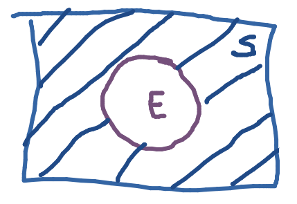
An event is a subset $E ⊆ S$ of the sample space $S$. The probability of the even $E$ is given by:
\[P(E)=\sum_{x\in E}P(x)\]
- $0 ≤ P(E) ≤ 1$ for every event $E$
- $P(\emptyset) = 0$ and $P(S) = 1$
Example - Fair Dice
If I roll a die three times, the event $E$ of rolling at least one 6 is given by:
- The set of sequences of length 4 over $\{1,\ldots,6\}$ containing at least one 6.
- $P(E)$ is the number of sequences containing at least one 6 divided by $6\times6\times6\times6=216$.
If we roll a fair die, then the event E of rolling an odd number is given by:
- The set $E=\{1,3,5\
- $P(E)=P(1)+P(3)+P(5)=\frac{1}{6}+\frac{1}{6}+\frac{1}{6}$ $=\frac{1}{2}$
Probability of Composed Events
- The complement of an event can be computed from the probability of the event.
- The union of events can be computed from the probabilities of the individual events.
Complement
Let $\neg E = S - E$. Then $P(\neg E)=1-P(E)$

Additionally, $S=\neg E\cup E$.
Proof
\[1=\sum_{x\in S}P(x)=\sum_{x\in E}P(x)+\sum_{x\in \neg E}P(x)\]
Thus,
\[\sum_{x\in\neg E}P(x)=1-\sum_{x\in E}P(x)\]
Example
What is the probability that at least one bit in a randomly generated sequence of 10 bits is 0?
- $S = \{0, 1\}^{10} =$ all sequences of 0 and 1 of length 10.
- For every $x ∈ S, P(x) = (\frac{1}{2})^{10} = \frac{1}{2^{10}}$.
- $E =$ all sequences of 0 and 1 of length 10 containing at least one 0.
- $\neg E=\{1111111111\}$
- $P(\neg E)=\frac{1}{2^{10}}$
- $P(E)=1-\frac{1}{2^{10}}$
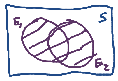
Union
\(P(E_1\cup U_2)=P(E_1)+P(E_2)-P(E_1\cap E_2)\)

Additionally, $\vert E_1\cup E_2\vert = \vert E_1\vert +\vert E_2\vert -\vert E_1\cap E_2\vert $
Proof
- $P(E_1)=\sum_{x\in E_1}P(x)$
- $P(E_2)=\sum_{x\in E_2}P(x)$
- $P(E_1\cup E_2)=\sum_{x\in E_1\cup E_2}P(x)$
Thus,
\[\begin{aligned}
P(E_1\cup E_2)=&\sum_{x\in E_1\cup E_2}P(x)\\
=&\sum_{x\in E_1}P(x)+\sum_{x\in E_3}P(x)\\
&-\sum_{x\in E_1\cup E_2}P(x)\\
=&P(E_1)+P(E_2)-P(E_1\cap E_2)
\end{aligned}\]
Example
Suppose I have a jar of 30 sweets:
| |
Red |
Blue |
Green |
| Circular |
2 |
4 |
3 |
| Square |
6 |
7 |
8 |
The sample space $S$ has 30 elements and if one chooses a sweet uniformly at random then then the probability for all $x\in S$ is:
\[P(x)=\frac{1}{30}\]
What is the probability of choosing a red or circular sweet?
- The probability that it is red is $\frac{2+6}{30}=\frac{8}{30}(P(R)=\frac{8}{30})$
- The probability that it is cicular is $\frac{2+4+3}{30}=\frac{9}{30}(P(C)=\frac{9}{30})$
Then $P(R\cup C)$ is the probability that the sweet is red or circular:
\[\begin{aligned}
P(R\cup C) &= P(R)+P(C)-P(R\cap C)\\
&= \frac{8}{30}+\frac{9}{30}-\frac{2}{30}\\
&=\frac{15}{30}=\frac{1}{2}
\end{aligned}\]
Disjoint Events
Assume that $E _1,\ldots,E_n$ are mutually disjoint events. So $E_i\cap E_j=\emptyset$ whenever $i\neq j$.
Then,
\[P(\bigcup_{i\leq i \leq n}E_i)=\sum_{1\leq i\leq n}P(E_i)\]
Example - Three Dice
Suppose that I roll a fair die three times:
- $S$ is the set of dequences of lengh three over $\{1,\ldots,6\}$ (or $\{1,\ldots,6\}^3$).
- $P(x)=\frac{1}{6\times6\times6}=\frac{1}{216}$ for all $x\in S$.
What is the probability that I roll at least one 6?
Let $E_1$: even that 1^st roll is a 6, $E_2$: event that 2^nd roll is a 6; $E_3$: event that 3^rd roll is a 6.
This means that we would like to know:
\[P(E_1\cup E_2 \cup E_3)\]
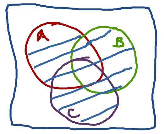
Computing the Probability of a Union of Three Sets
\[\begin{aligned}
P(A\cup B \cup C)=&P(A)+P(B)+P(C)\\
&-P(A\cap B)-P(A\cap C)\\
&- P(B\cap C)+P(A\cap B \cap C)\\
\end{aligned}\]

Additionally:
\[\begin{aligned}
\vert A\cup B \cup C\vert =& \vert A\vert + \vert B\vert +\vert C\vert\\
&-\vert A\cap B\vert -\vert A\cap C\vert -\vert B\cap C\vert\\
&+\vert A\cap B \cap C\vert
\end{aligned}\]
Example Continued
- $E_1$: even that 1^st roll is a 6.
- $E_2$: event that 2^nd roll is a 6.
- $E_3$: event that 3^rd roll is a 6.
We can calculate the answer with the equation from earlier:
\[\begin{aligned}
P(E_1\cup E_2 \cup E_3)=&P(E_1)+P(E_2)+P(E_3)\\
&-P(E_1\cap E_2)-P(E_1\cap E_3)\\
&- P(E_2\cap E_3)\\
&+P(E_1\cap E_2 \cap E_3)\\
=&\frac{36}{216}+\frac{36}{216}+\frac{36}{216}\\
&-\frac{6}{216}-\frac{6}{216}-\frac{6}{216}\\
&+\frac{1}{216}\\
=&\frac{91}{216}\approx0.42
\end{aligned}\]
Often we are interested in just part of the sample space. Conditional probability gives us a means of handling this situation.
Example
Consider a family chosen at random from a set of families having two children (but not having twins). What is the probability that both children are boys?
A suitable sample space $S=\{BB,GB,BG,GG\}$.
It is reasonable to assume that $P(x)=\frac{1}{4}$ for all $x\in S$.
Thus $P(BB)=\frac{1}{4}$.
Now you learn that the families were selected from those who have one child at a boys’ school. Does this change probabilities.
The new sample space $S’=\{BB,GB,BG\}$ and we re now looking for $P(BB\vert \text{at least one boy})+P(BB\vert S’)$
The vertical line is read given that.
Normalisation
$S’$ is a subset of $S$, so every outcome $x$ in $S’$ is also in $S$. It probability $P(x)\in S$ we can determine.
However, if we just take the sum of these probabilities, they will sum to less than 1.
We therefore normalise by dividing the probability $P(x)$ of the outcome $x$ in $S$ by the probability $P(S’)$ of $S’$ in $S$:
\[\begin{aligned}
P(BB\vert \text{at least one boy})&=P(BB\vert S')\\
&=\frac{P(BB)}{P(S')}\\
&=\frac{\frac{1}{4}}{\frac{3}{4}}\\
&=\frac{1}{3}
\end{aligned}\]
Conditioning
Assume now that evens $A$ and $B$ are given.
Assume we know that $B$ happens. So we want to condition on $B$. Thus, we want to know:
\[P(A\vert B)\]
This is the probability that $A$ occurs given that $B$ is know to occur.
So we want to know the probability $P(A\cap B)$. (as we know that $B$ occurs) after the conditioning on $B$.
We cant take $P(A\cap B)$ itself but have to normalise by dividing by the probability of the new sample space $P(B)$:
\[P(A\vert B)=\frac{P(A\cap B)}{P(B)}\]
Let $A$ and $B$ be events, with $P(B)>0$.
The conditional probability $P(A\vert B)$ of $A$ given $B$ is given by:
\[P(A\vert B)=\frac{P(A\cap B)}{P(B)}\]
View slide 27 for additional example.
Multiplication Rule
We can rewrite the previous equation like so:
\[P(A\cap B)=P(A\vert B)P(B)\]
Or like:
\[P(A\cap B)=P(B\vert A)P(A)\]
This rule can also be extended to more events:
\[\begin{aligned}
P(A\cap B\cap C)&=P(C\vert B\cap A)P(A\cap B)\\
&=P(C\vert A\cap B)P(B\vert A)P(A)
\end{aligned}\]
Example
Consider a family chosen at random from a set of families with just one pair of twins. What is the probability that both twins are boys?
Twins are either identical $I$ or fraternal $F$. We know that a third of human twins are identical:
\[P(I)=\frac{1}{3},P(F)=\frac{2}{3}\]
and
\[P(BB)=P(I\cap BB) + P(F\cap BB)\]
By the multiplication rule:
\[\begin{aligned}
P(I\cap BB)&= P(BB\vert I)P(I)\\
P(F\cap BB)&= P(BB\vert F)P(F)
\end{aligned}\]
The probability of being a girl of boy for fraternal twins will be the same as for any other two-child family. For the identical twins, the outcomes $BG$ and $GB$ are no longer possible thus:
\[P(BB\vert I)=\frac{1}{2},\ P(BB\vert F)=\frac{1}{4}\]
From this we obtain:
\[\begin{aligned}
P(BB)&=P(I\cap BB) + P(F\cap BB)\\
&=P(BB\vert I)P(I)+ P(BB\vert F)P(F)\\
&=\frac{1}{2}\times\frac{1}{3}+\frac{1}{4}\times\frac{2}{3}\\
&=\frac{1}{3}
\end{aligned}\]
In everyday language we refer to events that have nothing to do with each other as being independent.
Definition
Events $A$ and $B$ are independent if:
\[P(A\cap B)=P(A)\times P(B)\]
If $P(A)\neq 0$ and $P(B)\neq 0$, then the following are equivalent:
- $A$ and $B$ are independent.
- $P(B)=P(B\vert A)$
- $P(A)=P(A\vert B)$
See slides 31 for additional examples. This covers proving independence using the definition above.
Independence for More Than Two Events
For a finite set of events there are two different types of independence:
Pairwise Independence
$A_1,\ldots,A_n$ are pairwise independent if every pair of events is independent: for all distinct $k,m$
\[P(A_m\cap A_k)=P(A_m)P(A_k)\]
Mutual Independence
$A_1,\ldots,A_n$ are mutually independent if every event is independent of any intersection of the events: for all distinct $k,m$
\[P(A_{k1})\times\ldots\times P(A_{k_m})=P(A_{k_1}\cap\ldots\cap A_{k_m})\]
Pairwise independence doesn’t imply pairwise independence. Generally, if it isn’t stated, then we are talking about mutual independence.
To see the proof and example of why pairwise independence does not imply mutual independence see slide 37 onward. This example also shows examples of probability set notation.
If $P(A)>0$, then:
\[P(B\vert A)=\frac{P(A\vert B)\times P(B)}{P(A)}\]
Proof
We have:
- $P(A\cap B)=P(A\vert B)\times P(B)$
- $P(A\cap B)=P(B\vert A)\times P(A)$
Thus:
\[P(A\vert B)\times P(B)=P(B\vert A)\times P(A)\]
By dividing by $P(A)$ we get:
\[P(B\vert A)=\frac{P(A\vert B)\times P(B)}{P(A)}\]
Application - Diagnosis
Assume a patient walks into a doctor’s office complaining of a stiff neck. The doctor knows:
- Meningitis may cause a patient to have a stiff neck 50% of the time.
- The probability of having meningitis is $\frac{1}{50000}$
- The probability of having a stiff neck is $\frac{1}{20}$
What is the probability that the patient has meningitis?
Let $A$ be the event that the patient has a stiff neck and $B$ the event that they have meningitis:
\[\begin{aligned}
P(B\vert A)&=\frac{P(A\vert B)\times P(B)}{P(A)}=\\
\frac{\frac{1}{2}\times \frac{1}{50000}}{\frac{1}{20}}&=\frac{1}{5000}
\end{aligned}\]
You may not have the prior probability for $A$ (the observation). In this case you can use other things that you might know in this alternative form.
If $P(A)>0$, then:
\[\begin{aligned}
&P(B\vert A)=\\
&\frac{P(A\vert B)\times P(B)}{P(A\vert B)\times P(B)+P(A\vert \neg B)\times P(\neg B)}
\end{aligned}\]
Proof
It suffices to show:
\[P(A)=P(A\vert B)\times P(B)+P(A\vert \neg B) \times P(\neg B)\]
But this follows from:
\[\begin{aligned}
P(A)&=P((A\cap B)\cup (A\cap \neg B))\\
&=P(A\cap B)+P(A\cap\neg B)\\
&=P(A\vert B)\times P(B)+P(A\vert \neg B)\times P(\neg B)
\end{aligned}\]
Application - Diagnosis
Assume a drug test is:
- Positive for users 99% of the time.
- Negative for non-users 99% of the time.
Assume that 0.5% take the drug.
What is the probability that a person whose test is positive (event $A$) takes the drug (event $B$)?
We have:
- $P(A\vert B)=\frac{99}{100}$
- $P(\neg A\vert \neg B)=\frac{99}{100}$
- $P(B)=\frac{1}{200}$
Thus:
- $P(A\vert \neg B) =\frac{1}{100}$
- $P(\neg B) =\frac{199}{200}$
Thus:
\[\begin{aligned}
&P(B\vert A)=\\
&\frac{P(A\vert B)\times P(B)}{P(A\vert B)\times P(B)+P(A\vert \neg B)\times P(\neg B)}\\
&=\frac{99}{298}\approx0.33
\end{aligned}\]
Due to the low value it means that it is hard to take an action based on the test. This is as a result of the low value of the people who take the drug. This results in many false positives for those that don’t.
Let $(S,P)$ be a probability space. A random variable $F$ is a function $F:S\rightarrow\Bbb{R}$ that assigns to every $s\in S$ a single number $F(s)$.
In all these examples $S$ is the sample space and $P$ is the probability space.
- Neither a variable nor random.
- As it is the product of a function.
- English translation of variable casuale.
We still assume that the sample space is finite. Thus, given a random variable $F$ from some sample space $S$, the set of number $r$ that values of $F$ is finite as well.
The event that $F$ takes the value $r$, that is $\{s\vert F(s)=r\}$, is denoted $(F=r)$. the probability $(F=r)$ of the even $(F=r)$ is then:
\[P(F=r)=P(\{s\vert F(s)=r\})\]
Example 1
Let
\[S=\{\text{car, train, plane, ship}\}\]
Then the function $F:S\rightarrow \Bbb{R}$ defined by:
\[\begin{aligned}
F(\text{car})&=1\\
F(\text{train})&=1\\
F(\text{plane})&=2\\
F(\text{ship})&=2
\end{aligned}\]
is a random variable.
$(F=1)$ denotes the event $\{s\in S \vert F(s) =1\} = \{\text{car, train}\}$.
Defining a uniform probability space $(S,P)$ by setting:
\[P(\text{car})=P(\text{train})=P(\text{plane})=P(\text{ship})=\frac{1}{4}\]
This means that we are setting each event to have the same probability.
Then:
\[\begin{aligned}
P(F=1)=&P(\{s\in S \vert F(s)=1\})\\
=&P(\{\text{car, train}\})\\
=&\frac{1}{2}
\end{aligned}\]
Example 2
Suppose that I roll two dice. so the same sample space is:
\[S=\{1,2,3,4,5,6\}^2\]
and $P(ab)=\frac{1}{36}$ for every $ab\in S$.
Let
\[F(ab) = a+b\]
This means that we are investigating the sum of the two dice.
$F$ is a random variable. This variable maps the two values $ab$ to the sum $a+b$.
The probability that $F=r$ for a number $r$ (say, 12) is given by:
\[P(F=r)=P(\{ab\vert F(ab)=r\})\]
With this example:
\[\begin{aligned}
P(F=12)=&P(\{ab\vert F(ab)=12\})\\
=&P(66)\\
=&\frac{1}{36}
\end{aligned}\]
Random Variables
when defining a probability distribution $P$ for a random variable $F$, we often do not specify its sample space $S$ by directly assign a probability to the event that $F$ takes a certain value. Thus we directly define the probability:
\[P(F=r)\]
of the event that $F$ has the value $r$. Observe:
- $0\leq P(F=r)\leq 1$
- $\sum_{r\in \Bbb{R}}P(F=r)=1$
Thus, the events $(F=r)$ behave in the same way as outcomes of a random experiment.
Notation and Rules
Negation
We write $\neg(F=r)$ for the event $\{s\vert F(s)\neq r\}$. For example, assume the random variable $\text{Die}$ can take values $\{1,2,3,4,5,6\}$ and:
\[P(\text{Die}=n)=\frac{1}{6}\]
for all $n\in \{1,2,3,4,5,6\}$ (thus we have a fair die).
The $\neg(\text{Die}=1)$ denotes the event:
\[\begin{aligned}
&(\text{Die}=2)\vee (\text{Die}=3)\vee (\text{Die}=4)\vee\\
&(\text{Die}=5)\vee (\text{Die}=6)
\end{aligned}\]
We have the following complementation rule:
\[P(\neg(F=r))=1-P(F=r)\]
Intersection
We can write:
\[(F_1=r_1,F_2=r_2)\]
for $(F_1=r_1)$ and $(F_2=r_2)$. This takes two random variables
Union
Two represent the function OR we can write:
\[(F_1=r_1)\vee(F_2=r_2)\]
From this we can get the law from unions:
\[\begin{aligned}
P((r_1)\vee (r_2)) =& P(r_1)+P(r_2)\\
&-P(r_1,r_2)
\end{aligned}\]
Conditional Probability
if $P(F_2=r_2)\neq0$ then:
\[P(F_1=r_1\vert F_2=r_2)=\frac{P(F_1=r_1,F_2=r_2)}{P(F_2=r_2)}\]
This is the probability that $F_1=r_1$ given that $F_2=r_2$.
Product Rule
\(\begin{aligned}
P(F_1=r_1,F_2=r_2)=&P(F_1=r_1\vert F_2=r_2)\\
&\times P(F_2=r_2)
\end{aligned}\)
Symbols
Wo sometimes use symbols distinct from numbers to denote the values of random variables.
For example, for a random variable $\text{Weather}$ rather than using values $1,2,3,4$ we use:
\[\text{sunny, rain, cloudy, snow}\]
Thus, $(\text{Weather}=\text{sunny})$ denotes the event that it is sunny.
This is to say that random variable must give numbers as an output but we use symbols to represent these numbers.
To model a visit to a dentist, we use the random variables $\text{Toothache, Cavity}$ and $\text{Catch}$ (the dentist’s steel probe catches in the tooth) that all the take values 1 and 0 (for True or False).
For example, ($\text{Toothache}=1$) states that the person has toothache and ($\text{Toothache}=0$) states that the person does not have a toothache.
Examples of Probabilistic Models
To model a domain using probability theory, one first introduces the relevant random variable. We have seen two basic examples:
-
The weather domain could be modelled using the single random variable $\text{Weather}$ with values:
\[(\text{sunny},\text{rain},\text{cloudy},\text{snow})\]
-
The dentist domain could be modelled using the random variables $\text{Toothache, Cavity}$ and $\text{Catch}$ with values 0 and 1 for True or False. We might be interested in:
\[P(\text{Cavity}=1\vert\text{Toothache}=1,\text{Catch}=1)\]
Probability Distribution of a Single Random Variable
The probability distribution for a random variable gives the probabilities of all the possible values of the random variable.
For example let $\text{Weather}$ be a random variable with values:
\[(\text{sunny},\text{rain},\text{cloudy},\text{snow})\]
such that its probability distribution is given by:
- $P(\text{Weather}=\text{sunny})=0.7$
- $P(\text{Weather}=\text{rain})=0.2$
- $P(\text{Weather}=\text{cloudy})=0.08$
- $P(\text{Weather}=\text{snow})=0.02$
Assume the order of the values is fixed. The we write instead:
\[\mathbf{P}(\text{Weather})=(0.7,0.2,0.008,0.02)\]
Where the bold $\mathbf{P}$ indicates that the result is a vector of number representing the individual values of $\text{Weather}$.
We can write the values as a vector in the case that the properties are ordered.
Joint Probability Distribution
This is the case when you are using many random variables.
Let $F_1,\ldots,F_k$ be random variable. A joint probability distribution for:
\[F_1,\ldots,F_k\]
gives the probabilities:
\[P(F_1=r_1,\ldots,F_k=r_k)\]
for the event:
\[(F_1=r_1)\text{ and } \cdots \text{ and }(F_k=r_k)\]
that $F_1$ takes value $r_1$, $F_2$ take value $r_2$, and so on up to $k$ , for all possible values $r_1,\ldots,r_k$.
The joint probability distribution is denotes $\mathbf{P}(F_1,\ldots,K_k)$.
Example
A possible joint probabillity distribution $\mathbf{P}(\text{Weather, Cavity})$ for the random varables $\text{Weather}$ and $\text{Cavity}$ is given by the following table:
| $\text{Weather}=$ |
$\text{sunny}$ |
$\text{rain}$ |
$\text{cloudy}$ |
$\text{snow}$ |
| $\text{Cavity}=1$ |
0.144 |
0.02 |
0.016 |
0.02 |
| $\text{Cavity}=0$ |
0.576 |
0.08 |
0.064 |
0.08 |
For this to be plausible we should know that the two events are independent of each-other.
Full Joint Probability Distribution
A full joint probability distribution:
\[\mathbf{P}(F_1,\ldots,K_k)\]
is a joint probability distribution for all relavent random variables $F_1,\ldots,F_k$ for a domain of interest.
Every probability quesetion about a domain can be answered by tehf ull joint distributin because the probability of every evenint is a sum of the probabilities:
\[P(F_1=r_1,\ldots,F_k=r_k)\]
The $r_1,\ldots,r_k$ are often called data points or sample points.
Example
Assume the random variables $\text{Toothache, Cavity, Catch}$ fully describe a visit to a dentist.
The a full joint probability distribution is gien by the following table:
| |
$\text{Toothache}=1$ |
$\text{Toothache}=1$ |
$\text{Toothache}=0$ |
$\text{Toothache}=0$ |
| |
$\text{Catch}=1$ |
$\text{Catch}=0$ |
$\text{Catch}=1$ |
$\text{Catch}=0$ |
| $\text{Cavity}=1$ |
0.108 |
0.012 |
0.072 |
0.008 |
| $\text{Cavity}=0$ |
0.016 |
0.064 |
0.144 |
0.576 |
Marginalisation
Given an joint distribution $\mathbf{P}(F_1,\ldots,F_k)$, one can compute the marginal probabilities of the random variables $F_i$ by summing out the remaining variables.
For example:
\[\begin{aligned}
P(\text{Cavity}=1)&=0.108+0.012+0.072+0.008\\
&=0.2
\end{aligned}\]
is the sum of the entries in the first row of:
| |
$\text{Toothache}=1$ |
$\text{Toothache}=1$ |
$\text{Toothache}=0$ |
$\text{Toothache}=0$ |
| |
$\text{Catch}=1$ |
$\text{Catch}=0$ |
$\text{Catch}=1$ |
$\text{Catch}=0$ |
| $\text{Cavity}=1$ |
0.108 |
0.012 |
0.072 |
0.008 |
| $\text{Cavity}=0$ |
0.016 |
0.064 |
0.144 |
0.576 |
Conditional Distributions
We can also computer conditional distributions from the full joint distributions.
- We use the $\mathbf{P}$ notion for conditional distributions.
- $\mathbf{P}(F\ \vert\ G)$ gives the conditional distribution of $F$ given $G$ given by the probabilities $P(F=r\ \vert\ G=s)$ for all values $r$ and $s$.
- Using $\mathbf{P}$ notation, the general version of the product rule is as follows:
\[\mathbf{P}(F,G)=\mathbf{P}(F\ \vert\ G)\mathbf{P}(G)\]
This stands for the list of equations:
\[\begin{aligned}
P(F=r_1,G=s_1)=&P(F=r_1\ \vert\ G=s_1)\\
&\times P(G=s_1)\\
P(F=r_2,G=s_2)=&P(F=r_2\ \vert\ G=s_2)\\
&\times P(G=s_2)\\
\ldots=&\ldots
\end{aligned}\]
Probabilistic Inference
Probabilistic inference can be characterised as the computation of posterior probabilities:
\[\mathbf{P}(Q\ \vert\ E_1=e_1,\ldots,E_n=e_n)\]
for query variable $Q$ given observed evidence $e_1,\ldots,e_n$.
In principle, we can use the full joint distribution to do this.
Example - $\mathbf{P}(\text{Cavity}\ \vert\ \text{Toothache}=1)$
We want to compute the conditional probability distribution for $\text{Cavity}$ given the observation or evidence of $\text{Toothache}=1$.
Thus we want to compute:
- $P(\text{Cavity}=1\ \vert\ \text{Toothache}=1)$
- $P(\text{Cavity}=0\ \vert\ \text{Toothache}=1)$
We can easily obtain this using the table:
\[\begin{aligned}
P(C=1\ \vert\ T=1)&=\frac{P(C=1, T=1)}{P(T=1)}\\
&=\frac{0.12}{0.2}=0.6\\
\end{aligned}\]
\[\begin{aligned}
P(C=0\ \vert\ T=1)&=\frac{P(C=0, T=1)}{P(T=1)}\\
&=\frac{0.08}{0.2}=0.4
\end{aligned}\]
In this example $C$ is $\text{Cavity}$ and $T$ is $\text{Toothache}$.
The denominator 0.2 can be viewed as a normalisation constant $\frac{1}{\alpha}=5$ for the distribution $\mathbf{P}(\text{Cavity}\ \vert\ \text{Toothache}=1)$, ensuring that is adds up to 1.
This means that instead of completing the computation above we can consider this:
\[\begin{aligned}
\mathbf{P}(C\vert T=1)&=\alpha\mathbf{P}(C,T=1)\\
&= \alpha(0.12,0.08)\\
&=5(0.12,0.08)\\
&= (0.6,0.4)
\end{aligned}\]
In this case $\alpha$ is defined as a value that makes the sum of the vector 1. In this case it is 5.
Additionally, $C$ is $\text{Cavity}$ and $T$ is $\text{Toothache}$.
Combinatorial Explosion
This approach does not scale well: for a domain described by $n$ random variable taking $k$ distinct values each we face tow problems:
- Writing up the full joint distribution requires $k^n-1$ entries.
- The $-1$ in this case is as the full joint distribution adds to 1. To optimise we can not calculate the last value and just take the difference of the existing values and one.
- There are too many calculations
- How to we find the numbers (probabilities) for the entries?
- We don’t have enough raw data.
For these reasons, the full joint distribution in tabular form in not a practical tool for building reasoning systems.
Random variables $F$ and $G$ are independent if:
\[\mathbf{P}(F,G)=\mathbf{P}(F)\times\mathbf{P}(G)\]
That is, for all values $r$ and $s$:
\[P(F=r,G=s)=P(F=r)\times P(G=s)\]
As one’s dental problems do not influence the weather, the pairs of random variables are each independent:
- $\text{Toothache},\text{Weather}$
- $\text{Catch},\text{Weather}$
- $\text{Cavity},\text{Weather}$
Example - Weather and Dental Problems
The full joint probability distribution:
\[\mathbf{P}(\text{Toothache, Catch, Cavity, Weather})\]
has 32 entries. It contains four tables for the dentist variables and one for the four kinds of weather.
The number of entries comes from the $2\times2\times2\times4$ of the 2 outcomes for the 4 dentist variables and the 4 outcomes of the $\text{Weather}$ variable.
Thus we have:
- 8 probabilities for $(\text{Weather}=\text{sunny})$:
- $P(\text{Weather}=\text{sunny}, \text{Toothache}=r_1,$ $\text{Catch} =r_2,\text{Cavity}=r_3)$
- And so on for the other three weather types.
Clearly we can make the independence assumption that for any combination of values of the random variables $\text{Toothache, Catch, Cavity,}$ the probability for $\text{Weather}$. For example:
\[\begin{aligned}
& P(\text{Weather}=\text{sunny} \vert\\
& \text{Toothache}=r_1, \text{Catch} =r_2,\text{Cavity}=r_3)\\
=& P(\text{Weather}=\text{sunny})
\end{aligned}\]
for all $r_1,r_2,r_3\in\{0,1\}$.
Thus equivalently:
\[\begin{aligned}
& P(\text{Weather}=\text{sunny} \vert\\
& \text{Toothache}=r_1, \text{Catch} =r_2,\text{Cavity}=r_3)\\
=& P(\text{Weather}=\text{sunny})\times\\
&P(\text{Toothache}=r_1, \text{Catch} =r_2,\text{Cavity}=r_3)
\end{aligned}\]
for all $r_1,r_2,r_3\in\{0,1\}$.
This means that they are related proportionally.
We have seen that the join probability distribution
\[\mathbf{P}(\text{Weather, Toothache, Catch, Cavity})\]
can be written as:
\[\mathbf{P}(\text{Weather})\times\mathbf{P}(\text{Toothache, Catch, Cavity})\]
The 32-element table for four variables can be constructed from one 4-element table and an 8-element table.
Independence Analysis
Unfortunately this type of independence is very rare as generally things that you want to compare are inter-related. This is especially true within a single domain.
Conditional independence is much more prevalent and useful.
Conditional Independence
Random variable $G,F$ are conditionally independent given $H_1,\ldots,H_n$ if:
\[\begin{aligned}
\mathbf{P} (G,F\vert H_1,\ldots,H_n)=&\mathbf{P}(G\vert H_1,\ldots,H_n)\\
\times& \mathbf{P}(F\vert H_1,\ldots,H_n)
\end{aligned}\]
or, equivalently:
\[\mathbf{P} (G\vert F, H_1,\ldots,H_n)=\mathbf{P}(G\vert H_1,\ldots,H_n)\]
This is using the multiplication rule.
Example - Dentistry
In the dentist domain it seems reasonable to assert conditional independence of the variables $\text{Toothache}$ and $\text{Catch}$, given $\text{Cavity}$:
\[\begin{aligned}
&\mathbf{P}(\text{Toothache,Catch}\vert \text{Cavity})\\
&=\mathbf{P}(\text{Toothache}\vert \text{Cavity})\mathbf{P}(\text{Catch}\vert\text{Cavity})
\end{aligned}\]
or, equivalently:
\[\begin{aligned}
&\mathbf{P}(\text{Toothache}\vert \text{Cavity})\\
&=\mathbf{P}(\text{Toothache}\vert\text{Catch, Cavity})
\end{aligned}\]
graph TD
Cavity --> Catch
Cavity --> Toothache
This means that the cavity causes the toothache and if you have a cavity it is more likely that the steel probe catches. The lack of the arrow between toothache and catch mean that given that they have a cavity there is no relation between catching and the toothache.
Using conditional independence of $\text{Catch}$ and $\text{Toothache}$ given $\text{Cavity}$ we can compute the joint probability distribution:
\[\mathbf{P}(\text{Toothache, Catch, Cavity})\]
using only the probability distributions:
\[\begin{aligned}
&\mathbf{P}(\text{Toothache}\vert \text{Cavity}),\\
&\mathbf{P}(\text{Catch}\vert\text{Cavity}),\\
&\mathbf{P}(\text{Cavity})
\end{aligned}\]
The computation is as follows (using first multiplication rule and the conditional independence):
\[\begin{aligned}
&\mathbf{P}(\text{Toothache, Catch, Cavity})\\
=& \mathbf{P}(\text{Toothache,Catch}\vert \text{Cavity})\times \mathbf{P}(\text{Cavity})\\
=& \mathbf{P}(\text{Toothache}\vert \text{Cavity})\times \mathbf{P}(\text{Catch}\vert\text{Cavity})\\
&\times\mathbf{P}(\text{Cavity})
\end{aligned}\]
The number of probabilities needed is reduces to 5. Moreover, these probabilities can often be learned form data.
Towards Belief Networks
Conditional independence can be used to give concise representations of many domains.
A belief network (Bayesian network) is a graphical probabilistic model of domain in which nodes represent random variable and arc probabilistic dependence (often causality).
graph TD
Cavity --> Catch
Cavity --> Toothache
Informally, if there is an arc from a random variable $F$ to another random variable $G$ then $G$ depends on $F$. $F$ is called a parent of $G$. It is assumed that there are not cycles and that any random variable $G$ is conditionally independent of any non-parent variable $G’$ given the parents of $G$ if $G’$ cannot be reached by a sequence of arcs from $G$. For example, the graph above.
The full joint probability distribution is then given as:
\[\prod_{F\text{ in the network}} \mathbf{P}(F\vert \text{parents}(F))\]
The $\prod$ symbol means “the product of”.
In the example:
\[\begin{aligned}
\mathbf{P}(\text{Toothache}\vert \text{Cavity})&\times \mathbf{P}(\text{Catch}\vert\text{Cavity})\\
&\times\mathbf{P}(\text{Cavity})
\end{aligned}\]
As cavity has no parents then we can just take it’s probability.
Example - Student Exam Domain
Variables: $\text{Grade, Answers, Background, Works_hard}$
Then is seems reasonable to assume that:
- $\text{Works_hard}$ and $\text{Background}$ are independent.
- $\text{Grade}$ and $\text{Works_hard}$ are independent given $\text{Answers}$ and $\text{Grade}$.
- $\text{Background}$ are independent given $\text{Answers}$.
We represent this modelling of the domain using the Belief Network:
graph TD
Background --> Answers
w[Works_hard] --> Answers
Answers --> Grade
Example - Fire Alarm Domain
The fire alarm domain can be represented in the following graph:
graph TD
Tampering --> Alarm
Fire --> Alarm
Fire --> Smoke
Alarm --> Leaving
Leaving --> Report
Joint Probability Distribution
We want to know the joint probability distribution from:
\[\mathbf{P}(F\vert \text{parents}(F))\]
Given a Belief Network, we can always assume an ordering:
\[F_1,\ldots,F_n\]
of its random variables such that for all $i,j$:
\[F_i\rightarrow F_j \text{ implies } i<j\]
Using the examples we can order the random variables as follows:
-
The student exam domain:
 graph TD
 Background --> Answers
 w[Works_hard] --> Answers
 Answers --> Grade
$\text{Background, Works_hard, Answers, Grade}$
-
The fire alarm domain:
 graph TD
 Tampering --> Alarm
 Fire --> Alarm
 Fire --> Smoke
 Alarm --> Leaving
 Leaving --> Report
$\text{Tampering, Fire, Alarm, Smoke, Leaving,}$ $\text{Report}$
In these examples we can see that there are no return/backward dependencies from items in the right of the list to items in the left of the list.
According to the chain rule, given $F_1,\ldots,F_n$ we have for all $r_1,\ldots r_n$:
\[\begin{aligned}
& P(F_1=r_1,\ldots,F_n=r_n)=\\
& P(F_1=r_1)\times\\
& P(F_2=r_2\vert F_1=r_1)\times\\
& P(F_3=r_3\vert F_1=r_1,F_2=r_2)\times\\
& \cdots\\
& P(F_n=r_n\vert F_1=r_1,\ldots,F_{n-1}=r_{n-1})
\end{aligned}\]
Using bold $\mathbf{P}$ notation this reads:
\[\begin{aligned}
\mathbf{P}(F_1,\ldots,F_n)=&\mathbf{P}(F_1)\times\\
& \mathbf{P}(F_2\vert F_1)\times\\
& \mathbf{P}(F_3\vert F_1,F_2)\times\\
& \cdots\\
& \mathbf{P}(F_n\vert F_1,\ldots,F_{n-1})
\end{aligned}\]
This also means that $F_1$ must have no parents as it is first in the list. This further means that if there are cycles they must start without a parent.
As parents $(F_i)\subseteq\{F_1,\ldots,F_{i-1}\}$ conditional independence implies:
\[\mathbf{P}(F_i\vert F_1,\ldots F_{i-1})=\mathbf{P}(F_i\vert\text{parents}(F_i))\]
This is to say that only the parent of the values of $F_i$ are required in order to calculate the probability of $F_i$ given it’s parents.
This means that we can rewrite the equation before as:
\[\begin{aligned}
\mathbf{P}(F_1,\ldots,F_n)=&\mathbf{P}(F_1)\times\\
& \mathbf{P}(F_2\vert \text{parents}(F_2))\times\\
& \mathbf{P}(F_3\vert \text{parents}(F_3))\times\\
& \cdots\\
& \mathbf{P}(F_n\vert \text{parents}(F_n))
\end{aligned}\]
Example - Student Exam Domain
graph TD
Background --> Answers
w[Works_hard] --> Answers
Answers --> Grade
This graph gives the full joint probability distribution of:
\[\mathbf{P}(\text{Background, Works\_hard, Answers, Grade})\]
This can then be computed with:
\[\begin{aligned}
&\mathbf{P}(\text{Background})\times\\
& \mathbf{P}(\text{Works\_hard})\times\\
& \mathbf{P}(\text{Answers}\vert \text{Background, Works\_hard})\times\\
& \mathbf{P}(\text{Grade}\vert \text{Answers})
\end{aligned}\]
This method gives significantly less entries than calculating using a full joint probability table. E.g. in the fire alarm example we go from $2^6-1$ entries to 12 by using conditional probabilities.
Example - Fire Alarm Domain
graph TD
Tampering --> Alarm
Fire --> Alarm
Fire --> Smoke
Alarm --> Leaving
Leaving --> Report
In this set we are using the following abbreviations:
- $P(A\vert B)=P(A=1\vert B=1)$
- $P(\neg A \vert B ) = P(A=0\vert B=1)$
- and so on.
Assume the following (conditional) probabilities:
- $P(\text{Tampering})=0.02$
- $P(\text{Fire})=0.01$
- $P(\text{Smoke} \vert \text{Fire})=0.9$
- $P(\text{Smoke} \vert \neg\text{Fire})=0.01$
- $P(\text{Alarm} \vert \text{Fire}\wedge\text{Tampering})=0.5$
- $P(\text{Alarm} \vert \text{Fire}\wedge\neg\text{Tampering})=0.99$
- $P(\text{Alarm} \vert \neg\text{Fire}\wedge\text{Tampering})=0.85$
- $P(\text{Alarm} \vert \neg\text{Fire}\wedge\neg\text{Tampering})=0.0001$
- $P(\text{Leaving} \vert \text{Alarm})=0.88$
- $P(\text{Leaving} \vert \neg\text{Alarm})=0.001$
- $P(\text{Report} \vert \text{Leaving})=0.75$
- $P(\text{Report} \vert \neg\text{Leaving})=0.01$
Querying
If a report is observed, then the probability of fire and tampering go up:
- $P(\text{Fire})=0.01$ and $P(\text{Fire}\vert\text{Report})=0.2305$
- $P(\text{Tampering})=0.02$ and $P(\text{Tampering}\vert\text{Report})=0.399$
If, in addition, Smoke is observed, then probability of Fire goes up further but Tampering goes down:
-
$P(\text{Fire}\vert \text{Report}\wedge\text{Smoke})=0.964$
If you have two independent sources of information related to a subject in conjunction then you can expect the probability to increase dramatically.
-
$P(\text{Tampering}\vert \text{Report}\wedge\text{Smoke})=0.0284$
If, however, $\neg$Smoke is observed, then the probability of Fire goes down:
- $P(\text{Fire}\vert \text{Report}\wedge\neg\text{Smoke})=0.0294$
- $P(\text{Tampering}\vert \text{Report}\wedge\neg\text{Smoke})=0.501$
We can see from this that independent sources of evidence to make decisions are crucial.
For worked examples on querying see these videos.
Summary
- Belief network are representations of conditional independence in probabilistic models.
- Querying can often be done using exact inference.
- Sometimes exact inference is too hard. There are also approximate algorithms.
- Lots of research on learning belief networks from data. Either learning the conditional probabilities or even the structure of a belief network.
Learning is the process of converting experience into expertise or knowledge.
For a machine the input to a learning algorithms is training data (representing experience) and the output is some expertise, which usually takes the form of another computer program that can perform some task.
Types of Learning
Supervised Learning
The learner is presented with examples:
\[(x_1,L(x_1)),\ldots,(x_n,L(x_n))\in \mathcal{X}\times\mathcal{Y}\]
This is to say that it contains a list of pairs where the first element is data and the second is a provided label.
of labelled data $x_i$ $(L(x_i)$ is the label of $x_i$) and the task is to generalise the examples to a function $f:\mathcal{X}\rightarrow\mathcal{Y}$. If $\mathcal{Y}$ is finite, then $f$ is also called a classifier.
Unsupervised Learning
The learner aims to find structure (also called patterns) in data without using examples. Clustering data into similar ones is a typical unsupervised learning problem.
Reinforcement Learning
Learning from rewards or punishments in a dynamic setting in which an agent has a long-term goal (winning a game, driving a car). Different from supervised learning as actions of the learner are not directly classified.
Examples
Hand-Written Digit Recognition
Say that you are given a set of handwritten numbers. There are a set of labelled images and the rest are unlabelled.
An input image of 28 by 28 pixels is given as a vector $\vec x=(x_1,\ldots,x_{28\times28}$ of real numbers. Learn a classifier:
$f:\{\text{images}\}\rightarrow\{0,1,2,3,4,5,6,7,8,9\}$
Face Detection
Learn a classifier:
$f:\{\text{image windows}\}\mapsto \{\text{non-face, frontal face,}$ $\text{profile-face}\}$
Again a supervised learning problem:
- Start with training data:
- Image windows labelled with $\{\text{non-face, frontal face, profile-face}\}$.
- Generalise the training data to classifier $f$.
Spam Detection
Detect whether incoming email is pam or not.
A supervised learning problem:
Input data is word-count (e.g. word viagra in email indicated spam.)
Requires a learning system as “enemy” keeps innovating.
When do we Need Machine Learning?
- The problem’s complexity.
- The need for adaptivity.
Tasks that are too Complex to Program
- Tasks performed by animals/humans.
- There are numerous tasks that we human beings perform routinely, yet our introspection concerning how we do them is not sufficiently elaborate to extract a well defined program.
- Examples are given above.
- Machine learning programs achieve quite satisfactory results.
- Tasks beyond human capabilities.
- Another wide family of tasks that benefit from machine learning techniques are related to the analysis of very large and complex data sets.
- Examples include: astronomical data, weather prediction, web search engines.
- Meaningful information is buried in data archives that are way too large and too complex for humans to make sense of.
Adaptivity
- One limiting feature of programmed tools is their rigidity. Once a program has been written down and installed, it stays unchanged. However many tasks change over time or from one user to another.
- Machine learning tools (programs whose behaviour adapts to their input data) offer a solution to such issues; they are, by nature, adaptive to changes in the environment they interact with.
- Examples include individual handwritten text, spam detection, speach recognition.
Supervised Learning of Classifiers
Given:
- A set $\mathcal X$ of possible instances of be classified:
- Emails
- Hand-written digits
- Image windows
- A finite set $\mathcal Y$ of classes:
- $\{\text{spam, not spam}\}$
- Training data $(x_1,L(x_1)),\ldots,(x_n,(L(x_n))\in \mathcal X \times \mathcal Y$. $L(x_1)$ is called the label of $x_i$.
- A class of functions $\mathcal F$ from $\mathcal X$ to $\mathcal Y$ from with the classifier $f$ is selected.
Aim
-
Compute classifier $f\in \mathcal F$ such that:
\[f(x)\approx L(x_i)\]
This is to say that the computer makes a function that performs similarly to a function that a human would program.
for all training data $x_i(L(x_i))$ such that for new $x\in\mathcal X$:
\[f(x)=y\]
is a good prediction for the class of $x$.
Towards the Naive Bayes Classifier
One wants the learn a classifier $f:\mathcal X \rightarrow \mathcal Y$
We have training data:
\[x_i(L(x_i)),\ldots,(x_m,L(x_m))\]
For a new $x\in\mathcal X$, the classifier predicts $f(x)=y\in\mathcal Y$ if:
\[P(Y=y\vert x)\geq P(Y=y'\vert x)\]
for all $y’\in \mathcal Y$
You take the maximally probable hypothesis. This last line also means any $y’$ distinct from $\mathcal Y$.
Thus, in the derivation of the naive Bayes’ classifier we introduce a random variable $Y$ that takes values in $\mathcal Y$.
We also make the (vary common assumption that every elemen of $\mathcal X$ is givenby values $e_1,\ldots,e_n$ of features $E_1,\ldots,E_n$. We model those as random variables as well. Thus $P(Y=y\vert x)$ stands for:
\[P(Y=y\vert E_1=e_1,\ldots,E_n=e_n)\]
Our training data then takes the form:
\[(e^1_1,\ldots,e^1_n,y_1),\ldots,(e^m_1,\ldots,e^m_n,y_m)\]
Example - Playing Tennis
We assume we know the weather on a particular day, and want to predict whether Peter play Tennis on that day.
The classifier (or classes) are that Peter plays tennis or he doesn’t play tennis.
Also assume we have collected data on the weather on days on which Peter plays or does not play Tennis.
The features used then collecting the weather data are:
- The feature outlook with values: sunny, overcast, rain.
- The feature temp with values: hot, mild, cool.
- The feature humidity with values: high, normal.
- The feature wind with values: weak, strong.
For this set the instance is a day and it’s features are the ones listed above.
Assume we want to predict whether Peter plays Tennis on a day for which:
- outlook=sunny
- temp=cool
- humidity=high
- wind=strong
In what follows we write:
\[P(\text{sunny}\vert \text{Yes})\]
for
\[P(\text{outlook}=\text{sunny}\vert\text{PlaysTennis}=\text{Yes})\]
and so on for the remaining random variables and probabilities.f
We would like to estimate:
\[P(Y=y\vert E_1=e_1,\ldots,E_n=e_n)\]
which in the example is:
\[P(\text{Yes}\vert\text{sunny, cool, high, strong})\]
But how can we do this directly if in the training data there is no entry for a day on which the outlook is sunny, the temperature is cool, the humidity is high, and the wind is strong?
Towards the Naive Bayes Classifier
We use Bayes’ theorem
\[\begin{aligned}
&P(Y=y\vert E_1=e_1,\ldots,E_n=e_n)\\
&=\frac{P(E_1=e_1,\ldots,E_n=e_n\vert Y=y)P(Y=y)}{P(E_1=e_1,\ldots,E_n=e_n)}
\end{aligned}\]
As we only want to compare probabilities, it is sufficient to estimate:
\[P(E_1=e_1,\ldots,E_n=e_n\vert Y=y)P(Y=y)\]
for all $y\in \mathcal Y$.
Estimating Probabilities
Thus we want to estimate:
\[P(\text{sunny, cool, high, strong}\vert\text{Yes})P(\text{Yes})\]
and
\[P(\text{sunny, cool, high, strong}\vert\text{No})P(\text{No})\]
We can estimate $P(\text{Yes})$ by dividing the number of days on which Peter plays tennis by the total number of days; and we can estimate $P(\text{No})$ by dividing the number of days on which Peter does not play tennis by the total
number of days.
But as there are no entries for days on which the outlook is sunny, the temperature is cool, the humidity is high and the wind is strong; how can we estimate $P(\text{sunny, cool, high, strong}\vert\text{Yes})$?
Assume Conditional Independence
Then we can “estimate” $P(\text{sunny, cool, high, strong}\vert\text{Yes})$$P(\text{Yes})$
by $P(\text{sunny}\vert\text{Yes})$$P(\text{cool}\vert\text{Yes})$$P(\text{high}\vert\text{Yes})$$P(\text{strong}\vert\text{Yes})$$P(\text{Yes})$
and $P(\text{sunny, cool, high, strong}\vert\text{No})$$P(\text{No})$
by $P(\text{sunny}\vert\text{No})$$P(\text{cool}\vert\text{No})$$P(\text{high}\vert\text{No})$$P(\text{strong}\vert\text{No})$$P(\text{No})$
Probabilities such as $P(\text{sunny}\vert\text{Yes})$ can be estimated by dividing the number of days on which Peter plays tennis on which it is sunny by the toal number of days on which Peter plays tennis.
Prediction
Using the training data we estimate:
$V_{\text{Yes}}=P(\text{sunny}\vert\text{Yes})P(\text{cool}\vert\text{Yes})P(\text{high}\vert\text{Yes})$$P(\text{strong}\vert\text{Yes})P(\text{Yes})$
and
$V_{\text{No}}=P(\text{sunny}\vert\text{No})P(\text{cool}\vert\text{No})P(\text{high}\vert\text{No})$$P(\text{strong}\vert\text{No})P(\text{No})$
We estimate, for example,
- $P(\text{Yes})=\frac{9}{14}$
- $P(\text{No})=\frac{5}{14}$
- $P(\text{strong}\vert\text{Yes})=\frac{3}{9}$
and obtain:
\[V_{\text{Yes}}=0.0053,V_{\text{No}}=0.0274\]
Thus, the naive Bayes’ classifier predicts that Peter will not play tennis.
This does assume that all the random variables are independent which is not true as the elements of the weather are not independent. This is not an issue as this is only an estimate for comparison purposes.
Suppose we want to predict the class of the instance with features $(e_1,\ldots,e_n)$.
We assume $E_1,\ldots,E_n$ are independent given $Y$ and estimate:
\[V_y=P(Y=y)\prod^n_{i=1}P(E_i=e_i\vert Y=y)\]
The $\prod$ symbol means the product of.
for all $y\in \mathcal Y$ as follows:
- $P(Y=y)$ is estimated by the number of instance labelled with $y$ in the training data divided by the number of all instances in the training data.
- $P(E_i=e_i\vert Y=y)$ is estimated by the number of instances with feature $e_i$ labelled as $y$ in the training data divided by the number of all instances labelled with $y$ in the training data.
We then set:
\[f(e_1,\ldots,e_n)=y\]
for the $y$ for which $V_y$ is maximal (take the maximally probability hypothesis).
View side 27 onwards for an additional example about filtering spam emails.
Summary
- A supervised learning algorithm based on Bayes Theorem.
- It is called naive because it is assumed that the features are independent of each other, given the classification.
- Naive Bayes classifier works surprising well in practice even if the features are obviously not independent given the classification.
This classifier is an example of similarity based classifiers.
Similarity Measures
Assume that we can measure the similarity between items in the training data $\mathcal X$. For example:
Distance Measures
We measure similarity between data items using a distance measure $d$ which assigns to data item $x$, $x’$ a non-negative number:
\[d(x,x')\in\Bbb{R}\]
$d(x,x’)$ is called the distance between $x$ and $x’$
One typically requires that $d$ satisfies the following equations for metric spaces:
- $d(x,y)=0$ if and only if $x=y$ (identity indiscernibles).
- This means that if the distance is zero then they are the same thing.
- $d(x,y)=d(y,x)$ (symmetry).
- This means that opposites have equal distance.
- $d(x,y)+d(y,z)\geq d(x,z)$ (triangle equality).
- This means that the distance from $x\rightarrow z$ must be greater that the distance of $x\rightarrow y\rightarrow z$.
Distances for Items with Numerical Features
Numerous distance measures have been introduced. Of particular importance is the Euclidean distance which gives, in the two and tree dimensional case, the length of the straight line between points.
The Euclidean Distance:
\[d((e_1,\ldots,e_n),(f_1,\ldots,f_n))\]
between $(e_1,\ldots,e_n)$ and $(f_1,\ldots,f_n)$ is:
\[\sqrt{\sum^n_{i=1}(e_i-f_i)^2}\]
For $n=1$:
\[d(e,f)=\sqrt{(e-f)^2}=\left\vert e-f\right\vert\]
For $n=2$:
\[d((e_q,f_q),(e_2))=\sqrt{(e_1-f_1)^2+(e_2-f_2)^2}\]
This is an application of the Pythagorean theorem for straight line distances.
Distances for Items with Non-Numerical Features
Consider qualitative data such as:
| Day |
outlook |
temp |
humidity |
wind |
play |
| D1 |
sunny |
hot |
high |
weak |
No |
| D2 |
sunny |
hot |
high |
strong |
No |
| D3 |
overcast |
hot |
high |
weak |
Yes |
| D4 |
rain |
mild |
high |
weak |
Yes |
What should the distance between $D1$ and $D2$ (as far as the weather is concerned) be?
A natural distance measure in this case is the matching distance between values of features. This distance is equal to the number of features where $Di$ and $Dj$ do not coincide.
This can give:
- $d(D1,D2)=1$
- $d(D1,D4)=2$
Nearest Neighbour Classifier
Assume the data in $\mathcal C$ come with a distance measure $s(x,x’)\in\Bbb{R}$ which states how similar $x,x’\in\mathcal X$ are. Then the nearest neighbour classifier works as follows:
Given training data:
\[(x_1,L(x_1)),\ldots,(x_n,L(x_n))\]
for a new $x\in\mathcal X$ to be classifier, let $x_i$ be the element of the training set that is nearest to $x$:
\[d(x,x_i)\leq d(x,x_j), \text{for all } x_j\neq x_i\]
Then define the value $f(x)$ of the classifier $f$ by setting:
\[f(x)=L(x_i)\]
1: Input: training data (x0, L(x0)), ... , (xn, L(xn))
2:     new x ∈ X to be classified
3: for i = 0 to n do
4:     Compute distance d(x, xi)
6: endfor
7: return L(xi) such that d(x, xi) is minimal
A nearest neighbour classifier partitions $\mathcal X$ into regions. boundaries are equal distance from training points:

We can then split the classes and follow the lines along the split of the two regions. For a new item we would then classify it by the region that it falls into.

In this case you can see that the purple item falls into the blue class as it is in that section.
Problems
- The nearest neighbour classifier is very close to the training data.
- It does not generalise the training data.
- If the training data is noisy, then the classifier is noisy as well.
- If a spam email is erroneously labelled as non-spam, then all similar emails will also be classified as non-spam.
$k$-Nearest Neighbour Classifier
For $x$ to be classifier find $k$ nearest $x_{i_1},\ldots,x_{i_k}$ in the training data.
Classify $x$ according to the majority vote of their class labels.
For $k=3$:

The $k$ represents the number of closest labels you are taking into account.
1: Input: training data (x0, L(x0)), ... , (xn, L(xn))
2:     new x ∈  X to be classified
3:
4: for i = 0 to n do
5:     Compute distance d(x, xi)
6: endfor
7: Let xi1, ... , xik be the list of items such that
8:     d(x, xij) is among the k smallest distances
9: return label L which occurs most frequently in L(xi1), ... , L(xik) (majority vote)
Learning a “good” $k$
To learn a “good” $k$ divide labelled data into training data $T$ and validation data $V$.
This will result in the following two subsets of the labelled data:

The left is the training data and the right is the validation data.
The classification error of a classifier $f$ on a set of data items is the number of incorrectly classified data items divided by the total number of data items.
We are saying here that we want a $k$ such that new items added have the least classification error.
Let:
- $f_1$ be the 1-nearest neighbour classifier obtained from the training data $T$.
- $f_2$ be the 2-nearest neighbour classifier obtained from the training data $T$.
- and so on for $3,\ldots,m$.
Choose $f_k$ for which the classification error is minimal on the validation data (not the training data).
Generalisation
- The aim of supervised learning is to do well on test data that is not know during learning.
- Choosing the values for parameters (here $k$) that minimise the classification error on the training data is not necessarily the best policy.
- We want the learning algorithm to model true regularities in the data and ignore noise in the data.
Training and Validation Data - $k=1$

If we chose the value that was best for the training data then we can see here that we would almost always go for $k=1$. However, we want to be good generally so we optimise $k$ for the test data.
Training and Validation Data - $k=7$

You can see that although the error of the training data goes up the “general” error (on the validation data) goes down. We want to increase $k$ to minimise this value.
The line also gets smoother as $k$ increases as it is interpolating the data and removing noise.
Properties and Training
As $k$ increases:
- Classification boundaries become smother (possibly reflecting regularity in the data.
- Error on the training data can increase.
Summary
Advantages
- $k$-nearest neighbour is simple but effective.
- Decision surface can be non-linear.
- Only a single parameter, $k$, easily learned by cross validation.
Disadvantages
- What does nearest mean?
- Need to specify a distance measure.
- Computational cost.
- Must store and sear through the entire training set at test time.
Independence and Disjoints
-
$P(A\vert B)=0$ if $A,B$ are disjoint.
-
Unless $P(A)=0$, there are not independent.
Independence is about the dependence relation between evens however disjoint just means they don’t happen as the same time.
