COMP108 (Algorithms)

The lecturer for this subject is Prof. Prudence Wong. Email is pwong@liverpool.ac.uk.

Algorithms

An algorithm is a precise and concise set of instructions that guide you to solve a specific problem in a finite amount of time.

graph LR
Input --> Algorithm
Algorithm --> Output

The differences between algorithms and programs are as follows:

• In algorithms the content is more important than the form.
• Algorithms are free from grammatical Rules.
• Programs must follow syntax rules.
  • Form is important.

Pseudo Code

This is a logical code that doesn’t strictly follow the syntax of any individual programming language. They are useful for drafting algorithms.

Pseudo code uses a combination of english and code to make it more human readable.

Control Flow

The following conventions for pseudo code are preferred:

if <condition> then
	<statement>
else
	<statement>

for <variable> <- <value1> to <value2> do
	<statement>

while <condition> do
	<statement>

Blocks

Block in control sequences should be laid out like so:

begin
	<statement1>
	<statement2>
	.
	.
	.
end

or:

{
	<statement1>
	<statement2>
	.
	.
	.
}

Operations

• The % operator can be used in place of mod.

Other Notes

The use of a boolean variable to mark a significant event is called a flag variable. You can use this to mark a condition that has been met.

It is recommended that you draw a trace table of all the values at each iteration to find logical errors in your algorithms. You can also use them to find out what an algorithm does.

This lecture follows through some examples of solving particular problems in pseudo code. The slides for this lecture are available here.

Factors of $x$ but Not Factors of $y$

In this example we find the factors of $x$ and $y$ and subtract the elements in the $y$ list from the $x$ list.

Lowest Common Multiple

This example iterates through all numbers until it finds one that satisfies mod = 0 for both numbers.

Using breaks in a loop is not a good practice as it diminishes readability.

Efficiency matters as we want to make more ambitious code to leverage increases in computational power. If we didn’t optimise code then we’d be wasting resources.

Time Complexity Analysis

Timing execution time is not enough as it is not reproducible and wastes time.

We should identify some important operations and count how many times these operation need to be executed.

We can then change the input size and see how the time the algorithm takes changes.

Data vs Speed Increase

Assume this initial scenario:

• An algorithm takes $n^2$ comparisons to sort $n$ numbers.
• We need 1 second to sort 5 numbers (25 comparisons).

Now suppose that Computing speed increases by a factor of 100:

• This means in 1 second we can now do 2500 comparisons.
• This gives a result of 50 numbers vs the original 5.

We show here that an $n^2$ comparison algorithm gives a 10 times speed increase with a raw 100 times speed increase.

Important Operations

Here is an algorithm:

sum = 0
i = 1
while i <= n do
begin
	sum = sum  + i
	i++
end 
output sum

The important operation of summation is addition.

For this algorithm we need $2n$ additions (dependant on the input size of $n$).

Which Algorithm is Fastest?

This question may be dependant on the input size you may want to use several algorithms:

• $f_1(n) = n^2 -3n+6$
• $f_2(n) = 50n+20$

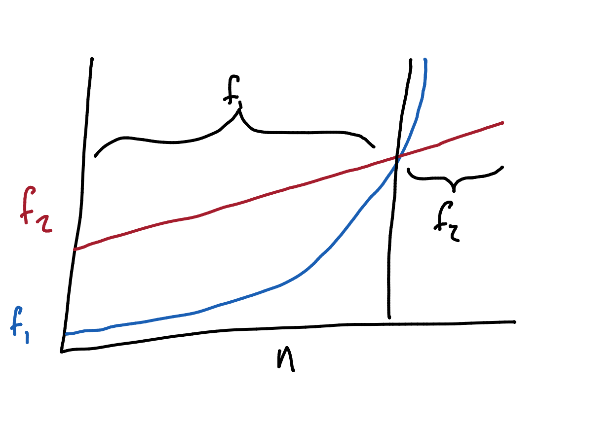
Generally you would want to choose the most efficient algorithm for when the input is maximal. In this example you would choose $f_2(n)$.

Growth Rate

Here are functions ordered by their growth rate:

• Constant
  • 1
• Logarithm
  • $\log n$
• Polynomial
  • $\sqrt n$
  • $n$
• Polynomial Logarithm (In-between each polynomial.)
  • $n\log n$
• Polynomial
  • $n^2$
  • $n^3$
• Exponential
  • $2^n$

In computer science $\log$ refers to $\log_2$.

Other Hierarchies

Comparing $\log^3n$ and $n$.

Identity: \(n\equiv 2^{\log_2n}\)

As $\log^3n$ is polynomial in terms of $\log n$ and $n$ (by the identity) is exponential in terms of $\log n$ the former is lower in the hierarchy.

Similarly, $\log^kn$ is lower than $n$ in the hierarchy, for any constant $k$.

Big-O Notation

\(f(n) =O(g(n))\)

Read as $f$ of $n$ is of order $g$ of $n$.

Roughly speaking, this means that $f(n)$ is at most a constant times $g(n)$ for all large $n$:

• $2n^3=O(n^3)$
• $3n^2=O(n^2)$
• $2n\log n=O(n\log n)$
• $n^3+n^2=O(n^3)$

When we have an algorithm, we can then measure its time complexity by:

• Counting number of operations in therms of the input size.
• Expressing it using big-O notation.

Powers

To find the time complexity of an algorithm look at the loops:

count = 0
for i = 1 to x do
	for j = 1 to y do
		for k = 1 to z do
			count = count + 1

For this loop the time complexity is $O(xyz)$. You can see that the variable relates to the time complexity.

Here is another example:

i = 1
while i <= n do
begin 
	j = i
	while j <= n do
		j = j + 1
	i = i + 1
end

The time complexity for this loop is $O(n^2)$. This is as a result of the time complexity of:

The highest term in this equation is $n^2$.

Logs

Here is another algorithm:

i = 1
count = 0 while i < n do
begin 
	i = i * 2
	count = count + 1
end
output count

This is the trace table for this algorithm:

• Suppose $n=8$

  Iteration	i before	i after	count
  Before Loop		1	0
  1	1	2	1
  2	2	4	2
  3	4	8	3

• Suppose $n=32$

  Iteration	i before	i after	count
  Before Loop		1	0
  1	1	2	1
  2	2	4	2
  3	4	8	3
  4	8	16	4
  5	16	32	5

We can see by comparing $n$ to the iterations that this algorithm is not linear.

To find the count that gives $n$ we would need to calculate:

Therefore this algorithm has logarithmic time complexity:

Don’t presume, when you see a loop, that the time complexity is polynomial.

For arrays, out of bounds means any index that is not in the range of the index.

When using arrays in pseudo code the following notation will be used:

arrayName[index]

Arrays in the notes will also be indexed from 1.

Sequential/Linear Search

Input

$n$ numbers stored in an array A[1..n], and a traget number key.

Output

Determine if key is in the array or not.

Algorithm

1. From i = 1, coparte key with A[i] one by one as long as i <= n.
2. Stop and report "Found" when key is the same as A[i].
3. Repeat and report "Not Found" when i > n.

Example

Found

Pseudo Code

i = 1
found = false
while i <= n AND found == false
begin
	if A[i] == key then
		found = true
	else
		i = i + 1	// Don't increment if number is found to save i.
end
if found == true then
	output "Found"
else
	output "Not Found"

Time Complexity

How many comparisons does this algorithm take?

• Best case:
  • The best case is where the key is the first element in the list.
  • $O(1)$
• Worst case:
  • The worst case is where the key is not in the array or the key is the last number.
  • $O(n)$

This method is a moire efficient way of searching but only when the sequence of numbers is sorted.

Input

A sequence of $n$ sorted numbers in ascending order and a target number key.

Method

1. Compare key with number in the middle.
2. Then focus on only the first half or the second half, dependant on whether key is smaller or greater than the middle number.
3. Reduce the amount of number to be searched by half.

Example

Go for lower if there is no middle. Consistency is key.

Found

If the key is not in the array you can conclude the number is not there when comparing to the last digit.

Pseudo Code

first = 1
last = n
found = false
while first <= last &&	found == false do
begin
	mid = floor((first + last) / 2)
	if A[mid] == key then
		found == true
	else if A[mid] > key then	// these two cases will trip first <= last
		last = mid - 1
	else A[mid] < key	
		first = mid + 1
end
if found == true then
	output "Found"
else
	output "Not Found"

Time Complexity

This search is generally quicker than linear search.

• Best case:
  • key is the middle number.
  • $O(1)$
• Worst case:
  • The key is not in the list.
  • At most $\lceil\log n\rceil+1$ comparisons.
    • $O(\log n)$

    This is as every comparison reduces the amount of numbers by at least half. We are asking: “How many times are we dividing $n$ by 2 to get 1?”

This assignment is based around memory management.

Paging/Caching

Two level virtual memory system

Slow memory contains more pages than fast memory called cache.

Requesting a page:

• If a page is already in cache.
  • Hit
• If page not in cache.
  • Miss.

In case of a miss, need to evict a page from cache to make room: eviction algorithms

Eviction Algorithms

No Eviction

Nothing is evicted with the cache containing exactly what it contains initially.

Example

• Cache: 20, 30, 10
• Sequence of Requests: 20, 30, 5, 30, 5, 20
• Output: hhmhmh (4h 2m)

Evict FIFO

In the case of a miss the first element in the cache will be evicted first. This is similar to a queue.

Example

• Cache: 20, 30, 10
• Sequence of Requests: 20, 30, 5, 30, 5, 20
• Output: hhmhhm (4h 2m)

Second row is after the request sequence.

Evict LFU (Least Frequently Used)

If there is more than one page with lowest frequency, evict the leftmost one.

Example

• Cache: 20, 30, 10
• Sequence of Requests: 20, 30, 5, 30, 5, 20
• Output: hhmhhh (5h 1m)

Evict LFD (Longest Forward Distance)

We look forward in the request queue and replace the item in the cache that is furthest forward. If there is more than one page with same position of next request $\infty$ evict, leftmost one.

Example

• Cache: 20, 30, 10
• Sequence of Requests: 20, 30, 5, 30, 5, 20
• Output: hhmhhh (5h 1m)

If the dataset is sorted in descending order then the first number is the maximum number.

This is excessive if set is unsorted.

Pseudo-code Examples

Maximum

i = 1
m = 0	# only works for +ve numbers; see next example
while i <= n do
begin
	if A[i] > m then
		m = A[i]
	i++
end
output m

Minimum

i = 1
m = A[1]	# initialise to the first number in the array
while i <= n do
begin
	if A[i] < m then	# this comparison is changed
		m = A[i]
	i++
end
output m

Time Complexity

The time complexity of this algorithm is:

This is as it iterates through every item in the list once.

Finding Location

i = 2	# location of second
loc = 1	# location of first
while i <= n do
begin
	if A[i] > A[loc] then
		loc = i
	i++
end
output loc and A[loc]

This will find the location of the first instance of the largest number.

To find the location of the last location you would use the following:

i = 2	# location of second
loc = 1	# location of first
while i <= n do
begin
	if A[i] >= A[loc] then
		loc = i
	i++
end
output loc and A[loc]

This will update if we come to a new instance of the maximum value.

Finding All Locations of Maximum

Find the first maximum:

m = A[1]
i = 2	# compare A[1] with A[2] in first iteration
while i <= n do
begin
	if A[i] > m then
		m = A[i]
	i = i + 1
end

Then print other locations of m:

i = 1
while i <= n do
begin
	if A[i] == m then
		output i
	i = i + 1
end
output M

Finding First and Second Maximums

m1 = max(A[1],A[2])	# ensure correct order
m2 = min(A[1],A[2])
i = 3	# skip comparing already compared
while i <= n do
begin
	if A[i] > m1 then
	begin
		m2 = m1
		m1 = A[i]
	end
	else if A[i] > m2 then
		m2 = A[i]
	i = i + 1
end 
output m1 and m2

Time Complexity

There is one loop with a constant number of comparisons. This gives a big-$O$ notation of:

Suppose we have data of daily rainfall for a year. Find the maximum monthly average rainfall over a year.

• Lets assume that there are $d$ days in a month and $m$ months in a year.

We could store rainfall data in a 2D array of size $m\times d$:

rainfall[i][j] stores rainfall of month $i$ and day $j$.

You can split the problem into the following questions:

1. What is the average rainfall of month $i$?
2. What is the maximum average?

Average of Month $i$

j = 1
sum = 0
while j <= d do
begin
	sum += rainfall[i][j]	# ask for i
	j++
end
average = sum / d

This is the nested portion of the loop. $i$ should be incremented outside.

Maximum of the Averages

m = 0
i = i
while i <= m do
begin
	sum = 0
	for j = 1 to d do
		sum += rainfall[i][j]
	average = sum / d
	if average > m then 
		m = average
	i++
end
output m

Time Complexity

The nested portion has a time complexity of $O(d)$. This is repeated $m$ times giving an overall time complexity of:

• Arrays - Alow random access to data.
• Queues - FIFO
• Stack - LIFO

Queues

There are two operations on a queue:

• Enqueue - Insert element to the tail.
• Dequeue - Delete element from the head.

The head points to the first element and the tail points to the location where data should be enqueued.

The actions are completed as follows:

• Enqueue
  • Save the data to Q[tail] and increment tail by 1.
• Dequeue
  • Retrieve data from Q[head] and increment head by 1.

Need to check if queue is empty before dequeue or full before enqueue.

Pseudo Code - Infinite Size

Enqueue(Q,x)
Q[tail] = x
tail++

Dequeue(Q)
if head == tail then # both pointers at same place
	Queue is EMPTY
else begin
	x = Q[head]
	head++
	return x
end

Pseudo Code - Limited Size

Enqueue(Q,x)
if tail > size then
	Queue is FULL
else begin
	Q[tail] = x
	tail++
end

Looping

In order to make use of free lower blocks the indexes must wrap around. This will give the following methods:

• Enqueue
  • After incrementing tail, if it exceeds size, then reset it to 1.
  • Same for checking full or not.
  • If indexes are from 0 to size - 1 you can use %.
• Dequeue
  • After incrementing head, if it exceeds size, then reset it to 1.
  • If indices are from 0 to size - 1, you can use %.

Stacks

The following are the operations on stacks:

• Push - Insert element tot he location 1 beyond top.
• Pop - Delete element from the top.

The stack has one pointer that points to the top-most data in the stack.

• Push
  • Increment top by 1 and save the data to S[top].
• Pop
  • Retrieve data from S[top] and decrement top by 1.

You need to check if the stack is empty before popping and the opposite for pushing.

Pseudo Code - Infinite Size

Push(S,x)
top++
S[top] = x

Pop(S)
if top == 0 then
	stack is EMPTY
else 
begin
	x = S[top]
	top--
	return x
end

Pseudo Code - Limited Size

Push(S,x)
if top == size then
	stack is FULL
else
begin
	top++
	S[top] = x
end

Post-fix Expressions with Stacks

You can use the stack to compute mathematical operations. This is the case if you use reverse Polish notation. This style of notation makes the precedence implicit.

Method

1. Rad the next token from the expressions which may be operator or operand.
2. If token is operand, PUSH it to stack.
3. If token is operator;
   • POP two operand from stack.
   • Operate on the two operands.
   • PUSH result back to stack.
4. If expression is not exhausted, go back to step 1.
5. If expression is exhausted, evaluation finished and answer is on top of stack.

Example

Evaluate 10 3 2 * - 5 *

Convert Infix to Postfix Expression Using Stack

Whenever an operator is popped, output it.

1. Read the next token from the expression which may be operator, operand, ( or ).
   • If token is operand, OUTPUT it.
   • If token is (, PUSH it on the stack.
   • If token is ), POP from the stack until matching (.
   • If token is operator, POP from stack until you see one of the following:
     • An operator with same/lower precedence.
     • An opening (.
     • The stack is empty.
   • PUSH the operator on stack.
2. If expression is not exhausted, go to step 1.
3. If expression is exhausted, POP rest of stack.

Linked lists are lists in which elements are arranges in a linear order. The order is determined by a pointer (rather than array indices).

Structure

Each node has a data field and one/two pointers linking to the next/previous element in the list.

Nodes with one pointer are called singly linked and ones with two are called doubly linked.

graph TD
subgraph node
prev --> a[ ]
data --> b[15]
next --> c[ ]
end

We refer to the three objects as: node.data, node.next and node.prev:

• If node is the last element, then node.next is NIL.
• If node is the first element, then node.prev is NIL.
• head points to the first node
• tail points to the last node.

The difference between linked lists and arrays is that you must follow the pointers to get to the data and can’t just go straight to a particular index.

graph LR
head --> prev1[ ]
subgraph 1
prev1[prev]
15
next1[next]
end
next1 --> prev2
subgraph 2
prev2[prev]
10
next2[next]
end
next2 --> prev3
subgraph 3
prev3[prev]
20
next3[next]
end
next3 --> tail

Traversing

Traversing and outputting each element of a linked list:

node = head
while node =/= NIL do
begin
	output node.data # output the data from this node
	node = node.next # go to next node
end

Searching

Searching if the value key is in a linked list:

node = head
found = false
while node =/= NIL AND found == false do
begin
	if node.data == "key" then
		found = true
	else # this keeps the node in the case that the element is found.
		node = node.next
end 
if found == true then
	output "Found!"
else output "Not found!"

Alternative

node = head
while node =/= NIL AND node.data =/= "key" do
	node = node.next
if node == NIL then
	output "Not found!"
else output "Found!"

Time Complexity

The time complexity of these two algorithms are:

Searching Sorted Lists

We are unable to use a binary search to find elements in a linked list as we have to walk the list. We are able to end the search if the data overshoots the requested data:

node = head
while node =/= NIL AND node.data < "key" do
	node = node.next
if node == NIL then # must check for NIL to avoid reading empty node
	output "Not found!"
else if node.data == "key" then
	output "Found!"
else output "Not found!"

Time Complexity

The time complexity of this algorithm is:

Insertion

Insertion to Head of List

List-Insert-Head(L,node)
	node.next = head
	node.prev = NIL
	if head =/= NIL then
		head.prev = node
	else // list was empty
		tail = node
	head = node

Insertion to Tail of List

List-Insert-Tail(L,node)
	node.next = NIL
	node.prev = tail
	if tail =/= NIL then
		tail.next = node
	else // list was empty
		head = node
	tail = node

Insertion in Middle

Suppose we want to insert a node after a node pointed to by curr.

# assume that curr is pointing to a node
List-Insert(L,curr,node)
	node.next = curr.next
	node.prev = curr
	curr.next.prev = node # points to new position from old next
	curr.next = node # point to new position from prev

This will not work if curr is at any end.

Time Complexity

The time complexity of:

• inserting to the head/tail of doubly linked list is $O(1)$.
• inserting to the head of singly linked list is $O(1)$.
• inserting to the tail of singly linked list is $O(n)$.
  • You may have to traverse the list if you don’t have an extra pointer for the last element in the list. If you do then it is $O(1)$
• inserting in a sorted doubly linked list is $O(n)$.
  • You have to search through the entire list in the worst case. The insertion is only $O(1)$.

Deletion from the Head of the List

Consider a list 15, 10, 20. We want to remove 15 and return it to the user.

List-Delete-Head(L)
	node = head
	if node =/= NIL then
	begin  // list wasn't empty
		head = head.next
		if head =/= NIL then
			head.prev = NIL
		node.next = NIL
	end
	return node

Deletion from the Tail of the List

Consider a list 15, 10, 20. We want to remove 20 and return it to the user.

List-Delete-Tail(L)
	node = tail
	if tail =/= NIL then
	begin // list wasn't empty
		tail = tail.prev
		tail.next = NIL
		node.prev = NIL
	end
	return node

Deletion from the Middle

Consider a list 15, 10, 20. We want to delete a node pointed to by curr and return the value.

// Assume that curr is pointing to a node
List-Delete(L, curr)
	curr.next.prev = curr.prev
	curr.prev.next = curr.next
	curr.next = NIL
	curr.prev = NIL
	return curr

Time Complexity

For a list with $n$ elements the following operations have the following time complexity:

• Traversing: $O(n)$
• Searching:
  • Unsorted: $O(n)$
  • Sorted: $O(n)$
• Insertion/Deletion:
  • Head/Tail: $O(1)$
  • Middle: $O(n)$
  • Finding the location may take $O(n)$ time.

Memory Management

• Memory needs to be allocated for a new node.
• We should free any object that is no longer used (after we delete a node).
• In some systems, a garbage collector is responsible for storage management.

Arrays v.s. Lists

• Arrays
  • Easy to access, one can access any element in a single access by its index.
  • Size needs to be predetermined, may waste space.
  • If we want to insert an element in the middle, needs to shift the rest.
• Linked Lists
  • Needs to traverse the list to access elements in the middle.
  • Does not need to predefine size, it’s flexible to add elements.
  • Once we find the location to insert, we can insert without moving the rest, only need to alter a few pointers.

Method

1. Starting from the first element, swap adjacent items if they are not in ascending order.
2. When last item is reached, the last item is the largest.
3. Repeat the above steps for the remaining items to find the second largest item.
4. When there is no change the list is sorted.

Example

Each table is one iteration:

No change, list is sorted.

Bold are being considered, italic are sorted.

Pseudo-Code

for i = n downto 2 do
	for j = 1 to (i - 1) do
		if (A[j] > A[j + 1]) then
			swap A[j] & A[j+1]
	end
end

Swapping Variables

Generally you need a temporary variable, otherwise you will overwrite your original data:

tmp = x
x = y
y = tmp

You can also recover the data this way without using a temporary variable:

x += y
y = x - y
x -= y

This method is less readable and may overflow if you have two very large numbers.

Time Complexity

The nested for loops give the following table:

This gives the following simplified equation:

We keep the highest power which gives the following big-O notation:

Cases

• In the best case bubble sort takes 0 swaps.
• In the worst case, bubble sort takes $O(n^2)$ times.

This time we will be looking at bubble sort in a linked list.

Linked List Pseudo Code

if head = NIL then
	Empty list and STOP
last = NIL
curr = head
while curr.next =/= last do
begin
	while curr.next =/= last do
	begin
		if curr.data > curr.next.data then
			swapnode(curr, curr.next)
		curr = curr.next
	end
	last = curr
	curr = head
end

Time Complexity Compared to Array

The time complexity is exactly the same as compared to using an array:

Method

1. Find minimum key from the input sequence.
2. Delete it from input sequence.
3. Append it to resulting sequence.
4. Repeat until nothing is left in the original sequence.

Example

Underlined is the current position, bold is the current smallest, and italic is sorted.

Pseudo-Code

This will give the following code when using while loops:

i = 1
while i <= n do
begin
	loc = i
	j = i + 1
	while j <= n do
	begin
		if A[j] < A[loc] then
			loc = j
		j++
	end
	swap A[i] and A[loc]
	i++
end

and the following for for loops:

for i = 1 to (n - 1) do
begin
	loc = i
	for j = (i + 1) to n do
		if A[j] < A[loc] then
		loc = j
	swap A[i] and A[loc]
end

Time Complexity

The nested for loops give the following table:

This gives the following simplified equation:

We keep the highest power which gives the following big-O notation:

Using Linked Lists

Pseudo-Code

if head ==  NIL then 
	Empty list and STOP
curr = head
while curr.next =/= NIL do
begin
	min = curr
	node = curr.next
	while node =/= NIL do
	begin
		if node.data < min dataq then
			min = node
		Node = node.next
	end 
	swapnode(curr,min)
	curr = curr.next
end

Time Complexity

The time complexity is exactly the same as compared to using an array:

Cases

• In the best case selection sort takes 0 swaps.
• In the worst case, selection sort takes $O(n^2)$ times.

Method

1. Look up the elements one by one.
2. Build up sorted list by inserting the element in the correct location.

Example

Bold is the number being considered and italic is the sorted list.

Pseudo-Code

for i = 2 to n do
begin
	key = A[i]
	loc = 1
	while loc < i AND A[loc] < key do
		loc++
	for j = i downto (loc + 1) do
		A[j] = A[j - 1]
	A[loc] = key
end

Time Complexity

The nested for loops give the following table:

From this we get the following big-O notation:

Using Linked Lists

Pseudo-Code

head = NIL
while thereIsNewNumber do
begin
	input number * create node
	node.data = num
	if head == NIL OR head.data > node.data then
	begin
		node.next = head
		head = node
	end
	else begin
		curr = head
		while curr.next =/= NIL AND curr.next <= node.data do
			curr = curr.next
		node.next = curr.next
		curr.next = node
	end
end

Time Complexity

The time complexity is exactly the same as compared to using an array:

Trees are linked lists with branches.

Definition

A tree $T=(V,E)$ consists of a set of vertices $V$ and a set of edges $E$ such that for any pair of vertices $u,v\in V$ there is exactly one path between $u$ and $v$:

graph TD
u((u)) --> y((y))
u --> v((v))
u --> x((x))
v --> w((w))

Equivalent Statements

1. There is exactly one path between two vertices in $T$.
2. $T$ is connected (there is at least one path between any two vertices in $T$) and there is no cycle (acyclic) in $T$.
3. $T$ is connected and removal of one edge disconnects $T$.
4. $T$ is acyclic and adding one edge creates a cycle.

5. $T$ is connected and $m=n-1$ (where $n\equiv \vert V\vert,m\equiv \vert E\vert$).

   This statement is proven next.

Statement 5 Proof

$P(n):$ If a tree $T$ has $n$ vertices and $m$ edges, then $m=n-1$.

By induction on the number of vertices.

Base Case

A tree with single vertex does not have an edge.

graph TD
a(( ))

$n=1$ and $m=0$ therefore $m=n-1$

Induction Step

$P(n-1)\Rightarrow P(n)$ for $n>1$?

1. Remove an edge from the tree $T$. By (3), $T$ becomes disconnected. Two connected components $T_1$ and $T_2$ are obtained, neither contains a cycle (otherwise the cycle is also present in $T$.

    graph LR
    u((u)) ---|remove| v((v))
   

   $u$ and $v$ are parts of two sub-trees ($T_1$ and $T_2$)that we are splitting.

2. Therefore, both $T_1$ and $T_2$ are trees.

   Let $n_1$ and $n_2$ be the number of vertices in $T_1$ and $T_2$.

   $\Rightarrow n_1+n_2=n$

3. By the induction hypothesis, $T_1$ and $T_2$ contains $n_1-1$ and $n_2-1$ edges, respectively.

   Therefore we can calculate that $m=(n_1-1)+(n_2-1)+1$. Simplified this is $m=n_1+n_2-1$. As $n=n_1+n_2$ we can simplify to $m=n-1$.

4. Hence $T$ contains $(n_1-1)(n_2-1)+1=n-1$ edges.

Rooted Trees

This is a tree with a hierarchical structure such as a file structure:

graph TD
/ --- etc
/ --- bin
/ --- usr
/ --- home
usr --- ub[bin]
home --- staff
home --- students
students --- folder1
students --- folder2
folder1 --- file1
folder1 --- file2
folder1 --- file3

The degree of this tree is 4 as / has the largest degree.

• The topmost vertex is called the root.
• A vertex $u$ may have some children below it, $u$ is called the parent of its children
• Degree of a vertex is the number of children it has.
• Degree of a tree is the maximum degree of all vertices.
• Vertex with no child (degree 0) is called a leaf.
• Vertices other than leaves/root are called internal vertices.
• Each child is the root of its own sub-tree.

• A binary tree is a tree where the degree is at most two.
• The two sub-trees are called left sub-tree and the right sub-tree (may be empty).

Traversing

There are three common ways to traverse a binary tree:

• Pre-order traversal (VLR)
  • Vertex, left sub-tree, right sub-tree.
• In-order traversal (LVR)
  • Left sub-tree, vertex, right sub-tree.
• Post-order traversal (LRV)
  • Left sub-tree, right-subtree, vertex

The difference is where the V appears.

Example

For the following tree you would gain the following traversals:

graph TD
r --- a
r --- b
a --- c
a --- d
d --- g
b --- e
b --- f
f --- h
f --- k

Pre-order

r, a, c, d, g, b, e, f, h, k

You can imagine this as following the left of the node.

In-order

c, a, g, d, r, e, b, h, f, k

You can imagine this as following the middle of the node.

Post-order

c, g, d, a, e, h, k, f, b, r

You can imagine this as following the right of the node.

Binary Search Tree

For a vertex with value $X$:

• Left child has value $\leq X$.
• Right child has value $> X$.

graph TD
60 --- 40
60 --- 90
40 --- 20
40 --- 50
20 --- 10
20 --- 30
90 --- 80
90 --- 110
80 --- 70
110 --- 100
110 --- 120

To search for a number go left if you want to go smaller and right if you want to go bigger.

In-order traversal gives the tree in ascending order.

Expression Tree

This tree represents a mathematical expression.

For the following expression:

In post-fix:

graph TD
*1[*] --- +
*1 --- 3((3))
+ --- 2((2))
+ --- *2[*]
*2 --- 5((5))
*2 --- 4((4))

Post-order traversal will give the post-fix representation.

Undirected Graphs

An undirected graph $G=(V,E)$ consists of a set of vertices $V$ and a set of edges $E$. Each edge is an unordered pair of vertices.

Unordered means that $\{b,c\}$ and $\{c,b\}$ refer to the same edge.

graph LR
a((a)) --- b((b))
a --- e((e))
a --- c((c))
a --- d((d))
b --- d
b --- c
b --- f
d --- e
e --- f

Terminology

For the following graph:

graph LR
u((u)) --- w((w))
u --- x((x))
u ---|e| v((v))
w --- v

• $u$ and $v$ are adjacent and are neighbours of each-other.
• $u$ and $v$ are endpoints of $e$.
• $e$ is said to be incident with $u$ and $v$.
• $e$ is said to connect $u$ and $v$.

The degree of a vertex $v$, denoted by $\deg(v)$, is the number of edges incident with it.

A loop contributes twice to the degree.

The degree of a graph is the maximum degree over all vertices.

Simple Graphs

An undirected graph is simple if:

• There is at most one edge between two vertices.
  • No self loops.

Multigraphs

• Allows more than one edge between two verices.

Directed Graphs

A directed graph $G(V,E)$ consists of the same as a directed graph. Each edge is an ordered pair of vertices.

Ordered means that the order of each pair of vertices refers to their direction.

graph LR
a((a)) --> b((b))
a --> e((e))
a --> c((c))
a --> d((d))
b --> d
b --> c
b --> f
d --> e
e --> f

This can be useful in referring to one-way paths.

Terminology

• A vertex is connected to another if there is a path from $a$ to $b$.
• In-degree of a vertex $v$ - The number of edges leading to $v$.

• Out-degree of a vertex $v$ - The number of edges leading away from $v$.

  The sum of the in and out degrees should always be equal and the same as two times the number of edges.

Example

There is an example on an undirected graph which proves:

The number of vertices with odd degree must be even.

Representation of Undirected Graphs

An undirected graph ca be represented by an adjacency matrix, adjacency list, incidence matrix or incidence list.

• Adjacency Matrix/List
  • The relationship between vertex adjacency (vertex vs vertex).
• Incidence Matrix/List
  • The relationship between edge incidence (vertex vs edge).

Adjacency Matrix/List

Adjacency matrix $M$ for a simple undirected graph with $n$ vertices is an $n\times n$ matrix:

• $M(i,j)=1$ if vertex $i$ and vertex $j$ are adjacent.
• $M(i,j)=0$ otherwise.

Adjacency list - each vertex has a list of vertices to which it is adjacent.

graph LR
a((a)) --- d((d))
a --- c((c))
b((b)) --- c
b --- d
c --- e((e))
c --- d
d --- e

The prior graph is represented in the following matrix:

$a$ to $b$ are listed left to right and top to bottom.

• The diagonals are always 0 on a simple graph.
• There is also diagonal symmetry as this is an undirected graph.
• The row/column will always add to the degree of the vertex.

This can also be represented in this list:

• $a\rightarrow c\rightarrow d$
• $b\rightarrow c\rightarrow d$
• $c\rightarrow a\rightarrow b\rightarrow d\rightarrow e$
• $d\rightarrow a\rightarrow b\rightarrow c\rightarrow e$
• $e\rightarrow c\rightarrow d$

The length of the list is the same as the number of edges.

If the graph has few edges and space is of a concern then the list is better.

Incidence Matrix/List

Incidence matrix $M$ for a simple undirected graph with $n$ vertices and $m$ edges is an $m\times n$ matrix:

• $M(i,j)=1$ if edge $i$ and vertex $j$ are incident.
• $M(i,j)=0$ otherwise.

Incidence list - each edge has a list of vertices to which it is incident with.

graph LR
a((a)) ---|2| d((d))
a ---|1| c((c))
b((b)) ---|3| c
b ---|4| d
c ---|7| e((e))
c ---|5| d
d ---|6| e

The prior graph is represented in the following matrix:

Vertices $a$ to $b$ are left to right and edges 1 to 7 are top to bottom.

• The columns sum to the degree of the vertex.
• The rows should sum to two for the two ends of the edge.

This can also be represented in this list:

• $1\rightarrow a\rightarrow c$
• $2\rightarrow a\rightarrow d$
• $3\rightarrow b\rightarrow c$
• $4\rightarrow b\rightarrow d$
• $5\rightarrow c\rightarrow d$
• $6\rightarrow d\rightarrow e$
• $7\rightarrow c\rightarrow e$

Representation of Directed Graphs

Adjacency Matrix/List

Adjacency matrix $M$ for a simple directed graph with $n$ vertices is an $n\times n$ matrix:

• $M(i,j)=1$ if $(i,j)$ if $i$ points to $j$.
• $M(i,j)=0$ otherwise.

Adjacency list - each vertex $u$ has a list of vertices pointed to by an edge leading away from $u$.

graph LR
a((a)) --> b((b))
c((c)) --> b
b --> d((d))
b --> e((e))
d --> e
c --> e

The prior graph is represented in the following matrix:

$a$ to $b$ are listed left to right and top to bottom.

• The diagonals are always 0 on a simple graph.
• There is no diagonal symmetry as this is an directed graph.
• The row/column will always add to the degree of the vertex.
• The sum of the matrix is the number of edges in the graph.

This can also be represented in this list:

• $a\rightarrow b$
• $b\rightarrow d\rightarrow e$
• $c\rightarrow b\rightarrow e$
• $d\rightarrow e$
• $e$

The length of the list is the same as the out-degree.

Incidence Matrix/List

Incidence matrix $M$ for a directed graph with $n$ vertices and $m$ edges is an $m\times n$ matrix:

• $M(i,j)=1$ if edge $i$ is leading away from vertex $j$.
• $M(i,j)=-1$ if edge $i$ is leading to vertex $j$.
• $M(i,j)=0$ otherwise.

Incidence list - each vertex $u$ has a list of vertices pointed to by an edge leading away from $u$.

graph LR
a((a)) -->|1| b((b))
c((c)) -->|2| b
b -->|3| d((d))
b -->|4| e((e))
d -->|5| e
c -->|6| e

The prior graph is represented in the following matrix:

Vertices $a$ to $b$ are left to right and edges 1 to 7 are top to bottom.

• There should be a -1 and 1 in each row.

This can also be represented in this list:

• $1\rightarrow a\rightarrow b$
• $2\rightarrow c\rightarrow b$
• $3\rightarrow b\rightarrow d$
• $4\rightarrow b\rightarrow e$
• $5\rightarrow d\rightarrow e$
• $6\rightarrow c\rightarrow e$

The order is significant.

• Paths
  • A number of nodes from one point to another.
• Circuits
  • If the start and end of the path is the same then it is a circuit.

Euler Circuits

A circuit that visits every edge once.

Vertexes can be repeated.

Not all graphs have an Euler circuit.

Conditions

• The graph must be connected.
  • This means that there must be no breaks in the graph.
• The degree of every vertex must be even.

Hamiltonian Circuit

Oppositely to an Euler circuit, this is a circuit that contains every vertex once.

This may not visit all edges.

This is a difficult problem to solve and will be reviewed later.

There are two main traversal algorithms: BFS and DFS. These have been covered in the following COMP111 lectures:

• COMP111 - Breadth First Search
• COMP111 - Depth First Search
• COMP111 - Properties of Searches

BFS with a Queue/Linked List

Example

Suppose $a$ is the starting vertex:

graph LR
a((a)) --- b((b))
a --- e((e))
a --- d((d))
b --- f((f))
e --- f
d --- h((h))
f --- c((c))
e --- k((k))
e --- g((g))
f --- k

This would generate the following queues when searching with BFS:

1. $\text{head}\rightarrow a\leftarrow\text{tail}$
2. $\text{head}\rightarrow b\rightarrow d\rightarrow e\leftarrow\text{tail}$
3. $\text{head}\rightarrow d\rightarrow e\rightarrow f\leftarrow\text{tail}$
4. $\text{head}\rightarrow d\rightarrow e\rightarrow f\leftarrow\text{tail}$
5. $\text{head}\rightarrow f\rightarrow h\rightarrow g\rightarrow k\leftarrow\text{tail}$
6. $\text{head}\rightarrow h\rightarrow g\rightarrow k\rightarrow c\leftarrow\text{tail}$
7. $\text{head}\rightarrow g\rightarrow k\rightarrow c\leftarrow\text{tail}$
8. $\text{head}\rightarrow k\rightarrow c\leftarrow\text{tail}$
9. $\text{head}\rightarrow c\leftarrow\text{tail}$

Every time an element is removed from the queue, it is added to the traversal:

BFS: $a,b,d,e,f,h,g,k,c$

Pseudo Code

unmark all vertices
choose some starting vertex s
mark s and insert s into tail of list L
while L is non-empty do
begin
	remove a vertex v from head of L
	visit v 	// print its data
	for each unmarked neighbour w of v do
		mark w and insert w into tail of list L
end

DFS with Stack

Example

Suppose $a$ is the starting vertex:

graph LR
a((a)) --- b((b))
a --- e((e))
a --- d((d))
b --- f((f))
e --- f
d --- h((h))
f --- c((c))
e --- k((k))
e --- g((g))
f --- k

This would generate the following stacks when searching with DFS:

1. $\mathbf a\leftarrow \text{top}$
2. $e,d,\mathbf b\leftarrow \text{top}$
3. $e,d,\mathbf f\leftarrow \text{top}$
4. $e,d,k,e,\mathbf c\leftarrow \text{top}$
5. $e,d,k,\mathbf e\leftarrow \text{top}$
6. $e,d,k,k,\mathbf g\leftarrow \text{top}$
7. $e,d,k,\mathbf k\leftarrow \text{top}$

8. $e,d,k\leftarrow \text{top}$

   Not added to path as it already exists.

9. $e,\mathbf d\leftarrow \text{top}$
10. $e,\mathbf h\leftarrow \text{top}$

11. $e\leftarrow\text{top}$

    Not added to path as it already exists.

Every time a unique element is popped from the stack, it is added to the traversal:

DFS: $a,b,f,c,e,g,k$

Pseudo Code

unmark all vertices
push starting vertex u onto top of stack S
while S is non-empty do
begin
	pop a vertex v from top of S
	if v is unmarked then
	begin
		visit and mark v
		for each unmarked neighbour w of v do
			push w onto top of S
	end
end

The process of the greedy algorithm is explained in this lecture:

• COMP111 - Informed Strategies

The main idea is to bin pack using the largest items first.

Greedy algorithm doesn’t always find an optimal solution but it is easy to implement.

Knapsack Problem

You want to steal the best items from a house optimising for:

• Least Weight
• Most Value

Formally this can be written like so:

Given $n$ items with weights $w_1,w_2,\ldots,w_n$, values $v_1,v_2,\ldots,v_n$ and a knapsack with capacity $W$.

Find the most valuable subset of items that can fit into the knapsack.

Exhaustive Algorithm

Approach:

• Try every subset of $n$ given items.
• Compute total wight of each subset.
• Compute total value of those subsets that do not exceed knapsack’s capacity.
• Pick the subset that has the largest value.

Analysis:

• There are $2^n-1$ subsets to consider.
  • This is exponential in $n$.

Example

Consider the following values:

• Item 1
  • $w=10$
  • $v=60$
• Item 2
  • $w=20$
  • $v=100$
• Item 3
  • $w=30$
  • $v=120$
• Knapsack
  • Capacity $=50$

One method of optimising would be to iterate through each combinations of subsets that fit in the knapsack and select the set with the most value:

An issue with this method is that the combinations grow exponentially with additional items.

Greedy Algorithm

Example

Consider the following values:

• Item 1
  • $w=10$
  • $v=60$
• Item 2
  • $w=20$
  • $v=100$
• Item 3
  • $w=30$
  • $v=120$
• Knapsack
  • Capacity $=50$

Pick the item with the next largest value if total weight $\leq$ capacity.

Result:

• Item 3 is picked, total value = 120, total weight = 30.
• Item 2 is picked, total value = 220, total wight = 50.
• Item 1 cannot be picked.

This happens to be optimal.

Time Complexity

First the values need to be sorted. This takes:

Completeness

This algorithm doesn’t always give an optimal solution. Using other modifiers like $\frac v w$ also won’t give optimal solutions.

Approximation Ratio

No matter the input, if a greedy algorithm has an approximation ratio of $\frac1 2$, it will always select a subset with a total value of at least $\frac 1 2$ of the optimal solution.

Minimum Spanning Tree (MST)

Given an undirected connected graph $G$:

• The edges are labelled by weight

Spanning tree of $G$:

A tree containing all vertices in $G$.

Minimum spanning tree of $G$:

• A spanning tree of $G$ with minimum weight.

Example

Undirected connected graph $G$:

graph LR
a ---|2| b
b ---|3| c
a ---|3| c
b ---|2| d
c ---|1| d

Spanning trees of $G$:

graph LR
a ---|2| b
b ---|3| c
b ---|2| d

graph LR
a ---|2| b
b ---|2| d
c ---|1| d

graph LR
b ---|3| c
a ---|3| c
c ---|1| d

There are $m\choose{n-1}$ (choose) possible spanning trees, where $m$ is the number of edges in the original graph and $n$ is the number of nodes.

Minimum spanning tree of $G$:

graph LR
a ---|2| b
b ---|2| d
c ---|1| d

This tree has the smallest total weight.

Kruskal’s Algorithm

The idea is to select edges from smallest to largest weight until the MST is made.

Example

graph LR
a ---|4| b
b ---|11| h
a ---|8| h
h ---|7| i
b ---|8| c
i ---|2| c
h ---|1| g
c ---|7| d
d ---|14| f
c ---|4| f
g ---|2| f
d ---|9| e
f ---|10| e

1. Arrange edges from smallest to largest weight.
2. Select edges from smallest to largest, provided that they don’t make a cycle.

This gives the following tree:

graph LR
a ---|4| b
a ---|8| h
i ---|2| c
h ---|1| g
c ---|7| d
c ---|4| f
g ---|2| f
d ---|9| e

Order of edges selected:

(g, h), (c, i), (f, g), (a, b), (c, f), (c, d), (a, h), (d, e)

This algorithm is greedy as it chooses the smallest wight edge to be included in the MST.

Pseudo Code

Given an undirected connected graph $G=(V,E)$:

T = Ø
E' = E	// E' is the set of all edges
while E' != Ø do
begin
	pick an edge e in E' with minimum weight
	if adding e to T does not form cycle then
		add e to T	// This is the same as T = T ∪ {e}
	remove e from E'	// This is the same as E' = E' \ {e}
end

Determining Whether Cycles are Formed

When we consider a new edge $e=(u, v)$, there may be three cases:

1. At most one of $u$ and $v$ is end point of an already chosen edge.
   • No cycle
2. $u$ and $v$ both belong to the same partial tree that has been already chosen.
   • Cycle
3. $u$ and $v$ belong to two separate partial trees that have been already chosen.
   • No cycle

Time Complexity

The time complexity is:

This will give a big-o notation of:

Optimising Pseudo Code

• You can stop earlier if you know that you have the correct number of edges.
• You can also presort the edges.

With these two the time complexity is:

Single-Source Shortest Paths

Consider a directed/undirected connected graph $G$:

• The edges are labelled by weight.

Given a particular vertex called the source:

• Find shortest paths from the source to all other vertices.

Example

Undirected connected graph $G$:

graph LR
a ---|2| b
b ---|3| c
a ---|3| c
b ---|2| d
c ---|1| d

Shortest Paths (Local Property)

• From $a$:

    graph LR
    a((a)) ---|2| b
    a ---|3| c
    b ---|2| d
  

• From $b$:

    graph LR
    a ---|2| b
    b((b)) ---|3| c
    b ---|2| d
  

• From $c$:

    graph LR
    b ---|3| c
    a ---|3| c
    c((c)) ---|1| d
  

• From $d$:

    graph LR
    a ---|3| c
    b ---|2| d((d))
    c ---|1| d
  

Dijkstra’s Algorithm

This algorithm assumes that the weight of edges are positive.

The idea is to choose the edge adjacent to any chosen vertices such that the cost of the part to the source is minimum.

Example

Suppose that $a$ is the source:

graph LR
a((a)) ---|5| b
a ---|7| c
b ---|10| h
c ---|2| h
c ---|7| e
e ---|5| h
e ---|5| f
f ---|1| h
c ---|2| d
a ---|10| d
d ---|4| e
f ---|3| g
d ---|3| g
h ---|2| g

1. Every vertex keeps 2 labels, initially as $(\infty, -)$:
   1. The weight of the current shortest path from $a$.
   2. The vertex preceding $v$ on that path.

    graph LR
    a((a)) ---|5| b["b: (∞, -)"]
    a ---|7| c["c: (∞, -)"]
    b ---|10| h["h: (∞, -)"]
    c ---|2| h
    c ---|7| e["e: (∞, -)"]
    e ---|5| h
    e ---|5| f["f: (∞, -)"]
    f ---|1| h
    c ---|2| d["d: (∞, -)"]
    a ---|10| d
    d ---|4| e
    f ---|3| g["g: (∞, -)"]
    d ---|3| g
    h ---|2| g
   

2. Each round:
   1. A vertex is picked, neighbours’ labels updated.
   2. Pick from all un-chosen vertices the one with smallest weight for the next round.

    graph LR
    a((a)) ===|5| b["b: (5, a)"]
    a -.-|7| c["c: (7, a)"]
    b ---|10| h["h: (∞, -)"]
    c ---|2| h
    c ---|7| e["e: (∞, -)"]
    e ---|5| h
    e ---|5| f["f: (∞, -)"]
    f ---|1| h
    c ---|2| d["d: (10, a)"]
    a -.-|10| d
    d ---|4| e
    f ---|3| g["g: (∞, -)"]
    d ---|3| g
    h ---|2| g
   

   Followed paths are shown as dotted.

   $a\rightarrow b$ has the minimum weight so is chosen in bold.

This continues until the following graph is reached:

graph LR
a((a)) ===|5| b["b: (5, a)"]
a ===|7| c["c: (7, a)"]
b -.-|10| h["h: (9, c)"]
c ===|2| h
c -.-|7| e["e: (13, d)"]
e -.-|5| h
e -.-|5| f["f: (10, h)"]
f ===|1| h
c ===|2| d["d: (9, c)"]
a -.-|10| d
d ===|4| e
f -.-|3| g["g: (11, h)"]
d -.-|3| g
h ===|2| g

You should record the history of label changes.

In the case of a tie there is no difference. You may want to go alphabetically.

Table Presentation

Pseudo Code

Each vertex $v$ is labelled with two labels:

• A numeric label $d(v)$ indicates the length of the shortest path from the source to $v$ found so far.
• Another label $p(v)$ indicates the next-to-last vertex on such a path.
  • This is the vertex immediately preceding $v$ on that shortest path.

Given a graph $G=(V,E)$ and a source vertex $s$.

for every vertex v in the graph do
	set d(v) = ∞ and p(v) = null
set d(s) = 0 and V_t = Ø and E_t = Ø
while V \ V_t != Ø do	// there is still some vertex left
begin
	choose the vertex v in V \ V_t with minimum d(u)
	set V_t = V_t ∪ {u} and E_t = E_t ∪ {(p(u), u)}
	for every vertex v in V \ V_t that is a neighbour of u do
		if d(u) + w(u, v) < d(v) then	// a shorter path is found
			set d(v) = d(u) + w(u, v) and p(v) = v
end

$V_T$ and $E_T$ are the immediate sub-trees of $V$ and $V$ respectively.

Time Complexity

The time complexity is:

This gives an overall big-o notation of:

The idea of divide and conquer is to divide a problem into several smaller instances of ideally the same size.

• The smaller instances are solved, typically recursively.
• The solutions for the smaller instances are combined to get a solution to the large instance.

Sum Example

Find the sum of all the numbers in an array. Suppose we have 8 numbers:

We can apply the following:

graph BT
1[4 6 3 2 8 7 5 1] -->|36| 0[ ]
10[4 6 3 2] -->|15| 1
11[8 7 5 1] -->|21| 1
100[4 6] -->|10| 10
101[3 2] -->|5| 10
1000[4] -->|4| 100
1001[6] -->|6| 100
1010[3] -->|3| 101
1011[2] -->|2| 101
110[8 7] -->|15| 11
111[5 1] -->|6| 11
1100[8] -->|8| 110
1101[7] -->|7| 110
1110[5] -->|5| 111
1111[1] -->|1| 111

Pseudo Code

For simplicity, assume that $n$ is a power of 2. We can then call the following algorithm by RecSum(A, 1, n):

Algorithm RecSum(A[], p, q)
	if p == q then
		return A[p]	// this is the base case, there is one value
	else
	begin	// this is the iterative step
		sum1 = RecSum(A, p, (p+q-1)/2)	// this finds the two sides of the midpoint
		sum2 = RecSum(A, (p+q+1)/2, q)
		return sum1 + sum2
	end

Minimum Example

This finds the minimum number in an array.

Pseudo Code

For simplicity, assume that $n$ is a power of 2. We can call the following algorithm by RecMin(A, 1, n):

Algorithm RecMin(A[], p, q)
	if p == q then
		return A[p]	// pointing to the same value
	else
	begin
		answer1 = RecMin(A, p, (p+q-1)/2)	// divide the array
		answer2 = RecMin(A, (p+q+1)/2, q)
		if answer2 <= answer2 then	// find minimum of returned values
			return answer1
		else
			return answer2
	end

Time Complexity of Divide and Conquer

The time complexity is:

This is as there are $n$ order 1 comparisons completed.

Method

1. Divide the sequence of $n$ numbers into two halves.
2. Recursively sort the two halves.
3. Merge the two sorted halves into a single sorted sequence.

It is easier to merge two sequences that are already sorted, compared to two non-sorted sequences.

How to Merge

To merge two sorted sequences we keep two pointers, one to each sequence.

1. Compare the two numbers pointed.
2. Copy the smaller one to the result and advance the smaller pointer.
3. Repeat steps 1. and 2.
4. When we reach the end of one sequence, simply copy the remaining number in the other sequence to the result.

Pseudo Code

For simplicity, assume $n$ is a power of 2.

• $A$ is the full array.
• $B$ is sorting array 1.
• $C$ is sorting array 2.

Algorithm Merge(B[1..p], C[1..q], A[1..(p+q)])
	i = 1, j = 1, k = 1
	while i <= p AND j <= q do
	begin
		if B[i] <= C[j] then	// B is smaller
			A[k] = B[i]
			i++
		else	// C is smaller
			A[k] = C[j]
			j++
		k++
	end
	if i == (p + 1) then	// B is empty
		copy C[j..q] to A[k..(p+q)]
	else	// C is empty
		copy B[i..p] to A[k..(p+q)]

Example

Consider the following variables:

• $B=\{10,13,51,64\}$
  • $p=4$
• $C=\{5,21,32,34\}$
  • $q=4$

The following iterations occur:

Time Complexity

• Each node takes $O(r)$ time when there are $r$ integers.
• Each level takes $O(n)$ time because total number of integer is $n$.
• There are $O(\log n)$ levels.

This gives an overall time complexity of:

This is faster than other algorithms that we have seen so far.

The formula for Fibonacci numbers is as follows:

Pseudo Code

This is a recursive implementation:

Algorithm F(n)
	if n == 0 OR n == 1 then
		return 1
	else
		return F(n-1) + F(n-2)

Time Complexity

To analyse the time complexity of calculating Fibonacci numbers, we use a mathematical tool called recurrence.

Let $T(n)$ denote the time to calculate Fibonacci number $F(n)$:

• $T(n-1)$: Time to calculate $F(n-1)$.
• $T(n-2)$: Time to calculate $F(n-2)$.
• $+1$: Time to add $F(n-1)$ and $F(n-2)$.
• When $n$ is 0 or 1 there is no needed to divide and the only time needed is to return the number 1.

A recurrence is an equation or inequality that describes a function in terms of its value on smaller inputs.

To solve a recurrence is to derive asymptotic bounds on the solution.

Solving Recurrence for Fibonacci Numbers

Suppose $n$ is even:

Suppose $n$ is odd:

The expressions being operated on are in bold.

Solving Recurrence for Merge Sort

\(T(n)=\begin{cases} 1 & \text{if } n= 1\\ 2\times T(\frac n 2)+n & \text{if } n> 1 \end{cases}\)

Solving the Recurrence

Summary

For the following recurrences, the following time complexities are true:

• $T(n)=2\times T\left(\frac n 2\right) +1$
  • $T(n)$ is $O(n)$.

  This is for finding sum/min/max.

• $T(n)=2\times T\left(\frac n 2\right) +n$
  • $T(n)$ is $O(n\log n)$.

  This is merge sort.

• $T(n)=2\times T(n-1) +1$
  • $T(n)$ is $O(2^n)$.

  This is Fibonacci numbers.

• $T(n)=T\left(\frac n 2\right) +1$
  • $T(n)$ is $O(\log n)$.

  This is for recursive binary search.

Dynamic programming allows for more efficient implantation of divide and conquer algorithms.

Fibonacci Numbers

This is the definition for the Fibonacci numbers:

and the code that we had before:

Algorithm F(n)
	if n == 0 OR n == 1 then
		return 1
	else
		return F(n - 1) + F(n - 2)

This code calculates particular Fibonacci numbers many times which is inefficient.

Memorisation

To improve on this we can memorise new Fibonacci numbers so that we don’t have to calculate them again:

1. Store $F(n)$ somewhere after we have computed its value.
2. Afterwards, we don’t need to re-compute $F(n)$ as we can retrieve its value from the memory.

Main Algorithm
	set v[0] = 1
	set v[1] = 1
	for i = 2 to n do
		v[i] = -1	// initialise all other values to -1
	output F(n)

Algorithm F(n)
	if v[n] < 0 then
		v[n] = F(n - 1) + F(n - 2)
	return v[n]

This significantly reduces the amount of calculation.

Compute $F(n)$ in Advance

The 2$^{nd}$ version still makes many function calls. Making many function calls negatively effects performance. To improve this we can compute the values from the bottom-up.

Algorithm F(n)
	set v[0] = 1
	set v[1] = 1
	for i = 2 to n do
		v[i] = v[i - 1] + v[v - 2]
	return v[n]

Summary

• Write down a formula that relates a solution of a problem with those of sub-problems:
  • $F(n)=F(n-1)+F(n-2)$
• Index the sub-problems so that they can be stored and retrieved easily in a table.
• Fill the table in some bottom-up manner:
  • Start filling the solution of the smallest problem.
  • This ensures that when we solve a particular sub-problem, the solutions of all smaller sub-problems on which it depends are available.

Consider the following assembly line:

• 2 assembly lines, each with $n$ stations ($S_{i,j}$: line $i$ station $j$).
• $S_{i,j}$ and $S_{2,j}$ perform the same task by time taken is different.
• $a_{i,j}$ - Assembly time at $S_{i,j}$.
  • On the node.
• $t_{i,j}$ - Transfer time from $S_{i,j}$.
  • On the arrow.

graph LR
subgraph Line1
11[5]
12[5]
13[9]
14[4]
end
subgraph Line2
21[15]
22[4]
23[3]
24[7]
end
Start --> 11
11 -->|0| 12
12 -->|0| 13
13 -->|0| 14
14 --> End
13 -->|1| 24
12 -->|4| 23
11 -->|2| 22
Start --> 21
21 -->|0| 22
22 -->|0| 23
23 -->|0| 24
24 --> End
23 -->|1| 14
22 -->|11| 13
21 -->|2| 12

Determine which stations to go in order to while minimising the total time through the $n$ stations.

Trees

You can represent all the possible paths in a tree structure:

• The nodes are labelled with the assembly time.
• The edges are labelled with the transfer time.

You can then minimise for time while removing branches from the tree.

Dynamic Programming

To avoid populating the entire tree you can use a dynamic programming approach. This is because we don’t need to try all the possible choices.

1. If we know that fastest way to get to $S_{1,n}$ and $S_{2,n}$.
   • The faster of these two is overall the fastest.
2. To find the fastest way to $S_{1,n}$ we need to know the fastest way to $S_{1,n-1}$ and $S_{2,n-1}$.
3. Similarly for $S_{2,n}$.
4. Generalising, we want the fastest way to get though $S_{1,j}$ and $S_{2,j}$ for all $j$.

Sub-Problems

• Given $j$, what is the fastest way to get to $S_{1,j}$?
• Given $j$, what is the fastest way to get to $S_{2,j}$?

Definitions:

• $f_1[j]$ - The fastest time to get to $S_{1,j}$.
• $f_2[j]$ - The fastest time to get to $S_{2,j}$.

The final solution is:

Sub-Problem 1

Given $j$, what is the fastest way to get to $S_{1,j}$:

• The fastest way to $S_{1,j-1}$, then directly to $S_{1,j}$:

  \[f_1[j-1]+a_{1,j}\]

• The fastest way to $S_{2,j-1}$, a transfer from line 2 to line 1 then to $S_{1,j}$:

  \[f_2[j-1]+t_{2,j-1}+a_{1,j}\]

Therefore we want:

Boundary case:

Sub-Problem 2

Given $j$, what is the fastest way to get to $S_{2,j}$:

• The fastest way to $S_{1,j-1}$, a transfer from line 2 to line 1 then to $S_{2,j}$:

  \[f_1[j-1]+t_{1,j-1}+a_{2,j}\]

• The fastest way to $S_{2,j-1}$, then directly to $S_{2,j}$:

  \[f_2[j-1]+a_{2,j}\]

Therefore we want:

Boundary case:

Example

For an example on two assembly lines view slide 15 onwards.

The summary is that you go from the beginning of the line to the end, keeping track of both sides, and choosing the least cost as you progress.

The expected table form would be like this:

$f_1[j]$ and $f_2[j]$ are the shortest paths to each respective node.

Pseudo Code

f1[1] = a11
f2[1] = a21
for j = 2 to n do
begin
	f1[j] = min{f1[j-1] + a1j, f2[j-1] + t2(j-1) + a1j}
	f2[j] = min{f2[j-1] + a2j, f1[j-1] + t1(j-1) + a2j}
end
f* = min{f1[n], f2[n]}

Time Complexity

The time complexity is:

as it loops through each node once and completes some $O(1)$ tasks.

For more assembly lines this time complexity is the same.