ELEC320 (Neural Networks)

Optimal Hyperplane

Support vector machines create a hyperplane that linearly separates a set of data. This is called the optimal hyperplane.

The equation of optimal hyperplane takes the form:

Support Vectors

Support vectors are the closes data-points in the dataset to the optimal hyperplane. They are used to determine the location of the hyperplane that separates the set.

Using the function for the optimal hyperplane we can say:

The euclidean distance of a support vector from the optimal hyperplane can be calculated by:

Non-Separable Patterns

We can either use a slack variable ($\xi$) if the data is close to linearly separable, or we can transform the data to become linear.

Kernels

We can project each patterns $\mathbf x_i$ to a new feature space of higher dimensionality (compared to the original input space) using a projection function $\phi$:

We can use various types of kernels but the general form of the kernel machine is:

Weight Update Function

where:

• $\lambda$ if the user-defined regularisation parameter:
  • $\lambda=0$ indicates that the input data is completely trustworthy.
  • $\lambda=\infty$ indicates that the dataset needs significant smoothing.

Radial Basis Functions vs. Multi-Layer Perceptrons

Universal Approximators

Given any function $f(x)=y$, we can approximate such a function using either network type.

• Radial Basis Functions Require a Matrix inverse to be taken. This is slow and doesn’t scale well.
• Despite the lengthy weight update process in MLP, they are preferred as it can be parallelised for large datasets.

Pattern Separability

A complex pattern-classification problem, cast in a high-dimensional space non-linearly, is more likely to be linearly separable than in a low-dimensional space.

This can be reduced to:

• We can use a non-linear function to transform our data so that it can be classified using a linear perceptron.

  This has the benefit of using a small network with less layers.

Let \(D=\{\mathbf x_1,\ldots,\mathbf x_N\}\) be a set of $d$-dimensional patterns which belong to either of two classes $C_1$ or $C_2$.

For each pattern $\mathbf x_i$ we define some real-valued functions $\phi_i(\mathbf x)$ for $i=1,\ldots,b$. This defines teh multivalued mapping:

A dichotomy (binary partition) of the samples in $D$ if $\phi$-separable if there is a vector $\mathbf w$ such that:

The hyperplane $\mathbf x^T\phi(\mathbf x)=0$ partitions the $b$-dimensional $\phi$-space to two sides. At the same time the $d$-dimensional input-space to two parts.

Hence instead of using straight lines to partition the space we could use the following:

• Planes
• Spheres/Circles
• Quadrics

This allows us to classify XOR using a linear perceptron instead of using a multi-layer one.

Interpolation

For a given set of $N$ $d$-dimensional points $\mathbf x_i$, and a corresponding set of associated vlues $y_i$, there is a function $F$ such that $F(\mathbf x_i)=y_i,\forall i$. This is to say there is a surface that passes through all the points in the dataset.

One way for solving this problem is with the method of radial basis functions (RBFs). We define a function:

The parallel brackets mean that we calculate the distance between the two points.

$\phi(\parallel x-x_i\parallel)$ is a RBF

A real-valued function whose value depends only on the distance between the input an some fixed point $x_i$.

Commonly Used RBFs

Gaussian Functions:

There are more but they won’t be used in this module generally.

RBF Neural Network

This network approximates the nearest neighbour approach. There is only one hidden layer that uses RBFs instead of a simple sum:

graph LR
x1["x1(n)"] --> ϕ1
x2["x2(n)"] --> ϕ2
xd["xd(n)"] --> ϕM
x1 --> ϕ2
x1 --> ϕM
x2 --> ϕ1
x2 --> ϕM
xd --> ϕ1
xd --> ϕ2
ϕ1 -->|w1| sum
ϕ2 -->|w2| sum
ϕM -->|wM| sum
sum --> y
ϕ0 -->|w0| sum
subgraph input
x1
x2
xd
end
subgraph hidden
ϕ1
ϕ2
ϕM
end
subgraph output
sum
end

The following functions are used:

Backpropagation Activation Functions

In multi-layer perceptrons we require activation functions with continuous gradients so that their derivatives are significant.

Using a threshold would not be acceptable as it isn’t continuous.

Both of the following functions create small derivatives when used in large networks. Leaky ReLU may be a better option in those applications.

Sigmoid

This is given by the following function:

The derivative of this function is:

This can be derived by working out the partial derivatives for $\frac{\partial\phi}{\partial z}$.

Hyperbolic Tangent

This function $\tanh$ is readily available and has range of $(-1, 1)$ as opposed to $(0, 1)$ for sigmoid.

We can combine it with the scalars $\alpha$ and $\beta$ like so:

It derivative is:

Backpropagation Training Modes

• Sequential training mode (also known as stochastic gradient descent) adjust weights after each input.
• Batch training mode sums the errors across all samples and adjusts the weights after running all the input patterns.

A combination of the two is called mini batch which has smaller batch sizes:

• This reduces storage requirements over batch training, produces better gradients than sequential and avoids local minima better than sequential.

Enhancing BP Learning Rate

We can use momentum ($\mu$) to enhance the learning rate $\eta$ without having trouble with local minima:

Solutions to Overfitting

There are several solutions to overfitting:

• Early Stopping
• Regularisation (smoothing the gradient)
  • Weight Decay
  • Penalisation of Derivatives
  • Weight Elimination
• Optimal Brain Surgeon (OBS):
  • Remove least significant connections during training.
• Dropout
  • Remove least significant connections during testing.

Early Stopping

This method splits the labelled data into three sets:

• Training Set

• Validation Set

  This is new.

• Testing Set

This method stops learning when validation error is at minimum. This stops the network learning noise and helps it be more generalised.

Backpropagation

To update the weights for a multi-layer perceptron we need to complete the following steps:

1. Feed Forward
2. Backwards Pass

The general formula to update the weights on a multi-layer perceptron is:

where:

• $\nabla_\mathbf wE$ is the gradient with respect to $E$.
• $\eta$ is the learning rate.

We also have the following functions available:

• Output error for the $j^{\text{th}}$ neuron:

  \[e_j(n)=d_j(n)-y_i(n)\]

• Output network error:

  \[E(n)=\frac12\sum_{j\in\text{output}}e^2_j(n)\]

• Average network error:

  \[E_\text{avg}=\frac1N\sum^N_{n=1}E(n)\]

• Induced local field (ILF):

  \[v_j(n)=\text{sum weights and measures}\]

• Neuron output:

  \[y_j(n)=\phi(v_j(n))\]

• Local gradient (for one node):

  \[\delta_j(n)=e_j(n)\times\underbrace{\phi'(v_j(n))}_\text{activation function gradient}\]

• Weight update function:

  \[\nabla_\mathbf WE=-\delta_j(n)y_i(n)\]

Backwards Pass

Consider the following key equations:

A (output neuron):

B (hidden neuron):

1 (weight difference):

and follow the steps:

1. Calculate the local gradients by using A and B for the output and hidden layers.
2. Use equation 1 to update the gradients connecting the $j^\text{th}$ and $k^\text{th}$ neurons.

Learn an OR function using the following perceptron:

graph LR
x1 --> w1
x2 --> w2
x0 --> w0
w0 --> n[neuron]
w1 --> n
w2 --> n
n --> ϕ
ϕ --> y

where:

• $W = [w_0, w_1, w_2] = [-1, 1, -2]$
• $\eta = \frac12$

$w_0$ is a bias and $w_1$ and $w_2$ are the two inputs to the neuron.

We want to adjust the weights until all the input patterns on $x_1$ and $x_2$ produce the correct outputs.

The general method is as follows:

1. Calculate the induced local field by calculating the dot product of the inputs and weights:

   \[\mathbf x \cdot \mathbf w =\text{ILF}\]

   For this example:

   \[\begin{bmatrix}-1 & 0 & 1\end{bmatrix} \cdot\begin{bmatrix}0 & 1 & 0\end{bmatrix}=0\]

2. Calculate $y$ by using the activation function:

   \[y=\phi(\text{ILF})\]

   The activation function in this case has a positive bias so pulls values $\geq0$ to $1$ and drops values $<0$ to $-1$:

   \[y=\phi(0) =1\]

3. For an input of $x_1=0, x_2=1$ we expect an output of $d=1$. We calculate the error $e$ by taking the difference between $d$ and $y$:

   \[\begin{aligned} e&=d-y\\ &=1-1\\ &=0 \end{aligned}\]

4. If the error is non-zero we adjust the weights by the following function:

   \[\mathbf w(n+1)=\mathbf w(n)+\eta e(n)\mathbf x(n)\]

   In this case where no adjustment is needed and $\eta=\frac12$:

   \[\begin{aligned} \mathbf w(n+1)&=\mathbf w(n)+\eta e(n)\mathbf x(n)\\ &=\begin{bmatrix}0\\1\\0\end{bmatrix}+\frac12\times 0\times\begin{bmatrix}-1\\0\\1\end{bmatrix}\\ &=\begin{bmatrix}0\\1\\0\end{bmatrix} \end{aligned}\]

Least Mean Square (LMS)

This is a sample by sample approach. The linear least square method would be a batch approach.

where:

• $\mathbf w$ - weight vector
• $\eta$ - learning rate
• $e$ - the error $(d-y)$
• $d$ - expected result
• $y$ - neron output
• $\mathbf x$ - input vector

This uses value from a simple single layer network:

graph LR
x1 --> w1
x2 --> w2
xp --> wp
w1 --> adder
w2 --> adder
wp --> adder
adder --> y

Perceptron

Rosenblatt’s Perceptrons are based on the McCulloch-Pitts neuronal modal. They are similar to linear neurons, but they have non-linear activations based on thresholding activations:

with:

This uses the following network:

graph LR
x1 --> w1
x2 --> w2
xp --> wp
w1 --> t[threshold θ]
w2 --> t
wp --> t
t -->|1| vj
vj -->|"ϕ(vj)"| yj

Learning

Learning is a process by which the free parameters of a NN are adapted through a process of stimulation by the environment in which the network is embedded.

Learning is defined in the following actions:

1. The network is stimulated by the environment.
2. It’s free parameters undergo changes to reflect this stimulation. (training mode)
3. The network responds in a new way to the environment, as a result of the changes in its internal structure. (online mode)

Learning Rules

Error Correction Learning

Assume that the $k^\text{th}$ neuron receives a signal vector $\mathbf x(n)$, where $n$ is the tiem variable of a discrete synaptic adaptation procedure. This signal can be the result of other neurons in the previous layers.

We can define the error in the signal by:

where:

• $y_k(n)$ - the neuron output signal.
• $d_k(n)$ - the desired output signal.

Learning is achieved by minimising a cost function $E(n)$ until the system reaches a steady-state.

An example of a cost function could be squared error:

We can iterate on our error to converge on the desired $d_k$ value.

The amount we change the weight is given by:

We can change $\eta$ to change the speed of convergence and overshoot.

Memory Based Learning

Under this model we gather a large amount of data for past experiences which are stored in memory as a set $D_\text{train}$:

where:

• $\mathbf x_i$ - the sample
• $d_i$ - the desired response

In a graph of this data, we classify new data by choosing the nearest neighbour to the new data.

To get a better response we may use $n$-nearest-neighbour where we average the response of the $n$ neighbours.

Hebbian Learning

A Hebbian synapse is defines as a time-dependent, highly local and strongly interactive mechanism to increase synaptic efficiency:

• If neurons on either side of the synapse are activated simultaneously, then the strength of that synapse should be selectively increased.
• If the activation is asynchronous, then the synapse should be weakened.

This section is unfinished.

Competitive Learning

The output neurons compete amongst themselves to become active, as opposed to other learning rules where more than one neuron can be active.

This is better suited to classification problems as only one neuron is allowed to fire.

This section is unfinished.

Boltzmann Learning

Learning Paradigms

Credit/Blame (Credit Assignment Problem)

Supervised

Unsupervised Learning

Reinforcement Learning

Neuron Scheme

Each neuron is an information processing unit. Basic elements are:

• Synapses/Connections - Characterised by a weight $w_i$ and a signal $x_i$.
• Adder - Sums the input signals from the weighted synapses.
• Bias - $b_k$ is added to the sum.
• Activation function $\phi$ - Usually a non-linear function that produces the final output $y_k$.

graph LR
x1 -->|w1| n[Neuron]
x2 -->|w2| n
xn -->|wn| n
b["bias (bk)"] --> n
n -->|vk| af["Activation Function (phi(v))"]
af --> output["output (yk)"]

Where:

• $\mathbf w^T_k=[x_{k0},\ldots,w_{km}]$
• $\mathbf X=[x_0, \ldots,x_m]$

Types of Activation Functions

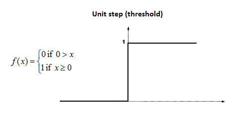
Threshold/Heavyside Function

¹

This has a binary output:

• Limited to binary classification only.
• No gradient information.

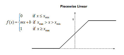
Piece-wise Linear Function

¹

• Narrow window of non-saturation.

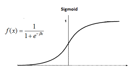
Sigmoid & Hyperbolic Tangent Functions

The following is a sigmoid function:

¹

there is also another s-shaped continuous function using $\tanh$.

Their ranges are:

• Sigmoid: 0 to 1
• $\tanh$: -1 to 1

or

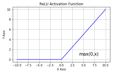
Rectified Linear Unit (ReLU)

²

Most common choice in state-of-the-art neural networks (deep learning):

• Non-linear
• Variants include leaky ReLU:
  • Has a shallow negative gradient when $v<0$.

Network Architectures

Single-layer Feed-forward Network

³

One input layer of source nodes that project directly onto the output computation.

There are no cycles allowed.

The output can be calculated using the following function:

Multi-layer Feed-forward Network

⁴

Has additional hidden layers in-between the input and output. These provide a more capable network:

• Typically the neurons of each layer take the previous layer as their input.
• Still no cycles.

The output can be calculated using the following function:

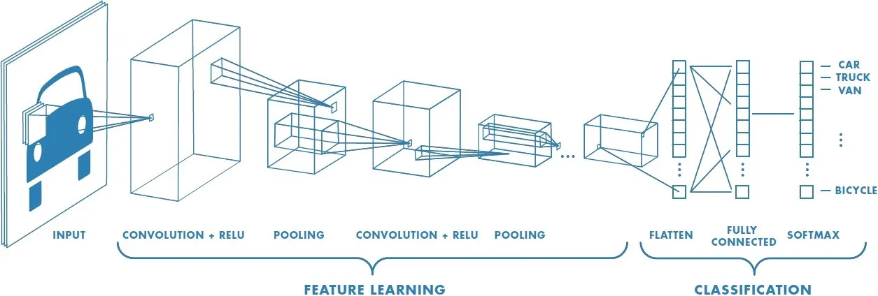
Convolutional Neural Networks (CNNs)

⁵

A class of multi-layer feed-forward network with a special type of local connections:

• Widely used for image classification.
• A convolution is used to gain deeper understanding of the image.

Recurrent Networks

These have feedback loops which form cycles in the graph:

• Feedback loops involve connections with unit-delay elements $z^{-1}$, which together with nonlinear activations enable the nonlinear dynamic behaviour of the network.

We can calculate the output of a recurrent, no hidden, delay one, self feedback network with the following:

Knowledge Representation

The primary task of a NN is to learn it’s environment. To accomplish this, we need to feed it with environment knowledge, which is based on:

• Observations - These are often noisy, contain errors and have redundant/missing information.
  • These can be labelled or unlabelled with the ground truth for that sample.

Training Dataset Example

A set ${{x_i, y_i}}, i=1,2,\ldots$ of experimentally acquired data is referred as a training dataset:

• OCR:
  • $x$ = Pixel values or curves.
  • $y$ = A, B, C, …

Training Process

1. Choose a subset of the available observations as a training dataset to teach the NN.

   This set should be diverse and representative of data used in production.

2. Choose an appropriate architecture, with as many input nodes as the length of the input feature vector $x$ and output nodes needed for the output $y$.
3. Train the network on the training dataset.
4. Test the network with the remaining data.

Brains and (A)NNs

The brain is:

• Highly Complex
• Non-linear
• Massively parallel

ANNs (artificial neural networks) are biologically inspired analogues of the brain and are based on primitive neuron components.

Neuron Structure

Synapses

Facilitate learning via creation of new, and modification of existing ones.

Axons

Signal transmission structures

Dendrites

Receptive structures

We can simulate a neuron with the following strucutre:

graph LR
x1 -->|w1| n[Neuron]
x2 -->|w2| n
xn -->|wn| n
n --> output

Each input has a weight and is summed as it enters the neuron to form the output:

We can then apply a threshold to the output if we want a binary output from the neuron.

Advantages of ANNs

• Non-linearity
• Input-to-output Mapping
• Adaptivity
  • NN can be retrained to adapt to solve a changing task or be adapted to a similar one.
• Evidential Response
  • A confidence can be provided as to whether the output is correct.
• Contextual Information
  • Knowledge is integrated into the network. Each neuron is affected by all others; local processing and global awareness.
• Fault Tolerance
  • When small damage occurs, the network usually degrades gracefully.
• Uniformity of Analysis and Design
  • NNs are composed of similar components. This allows for modularity and use of mathematics for learning and network analysis.
• Neuro-biological Analogy
  • As the system is already implemented in nature. The system is proven.

Using Machine Learning

Consider we want to use a NN to classify fish based on their lightness and width. We can use the following feature vector to represent each fish:

Where:

• $x_1$ is lightness
• $x_2$ is width

Based on a set of training samples, the neural network could produce the following decision boundary by use of it’s weights:

From this training we may observe the following phenomenon:

• Under-fitting
  • A machine learning model is not complex enough to accurately capture relationships between a dataset’s features and the target variable.
• Over-fitting
  • The model is too closely fit to a limited set of data points and does not generalise well to unseen data points.