Neural Network Structure

ELEC320 Lectures 2023-02-03

Neuron Scheme

Each neuron is an information processing unit. Basic elements are:

Synapses/Connections - Characterised by a weight $w_i$ and a signal $x_i$.
Adder - Sums the input signals from the weighted synapses.
Bias - $b_k$ is added to the sum.
Activation function $\phi$ - Usually a non-linear function that produces the final output $y_k$.

graph LR
x1 -->|w1| n[Neuron]
x2 -->|w2| n
xn -->|wn| n
b["bias (bk)"] --> n
n -->|vk| af["Activation Function (phi(v))"]
af --> output["output (yk)"]

\[\begin{aligned} v_k&=\sum^m_{j=0}w_{kj}x_j\\ &=\mathbf w^T_k\mathbf X\\ y_k&=\phi(v_k) \end{aligned}\]

Where:

$\mathbf w^T_k=[x_{k0},\ldots,w_{km}]$
$\mathbf X=[x_0, \ldots,x_m]$

Types of Activation Functions

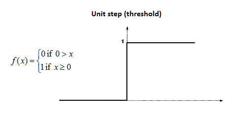
Threshold/Heavyside Function

Threshold function graph ¹

This has a binary output:

\[\phi(v)\begin{cases}1&\text{if}&v\geq0\\0&\text{if}&v<0\end{cases}\]

Limited to binary classification only.
No gradient information.

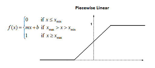
Piece-wise Linear Function

Piecewise linear function graph ¹

\[\phi(v)=\begin{cases}1 & \text{if} &v\geq\frac12\\v+\frac12&\text{if}&-\frac12<v<\frac12\\0&\text{if}&v\leq-\frac12\end{cases}\]

Narrow window of non-saturation.

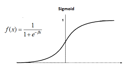
Sigmoid & Hyperbolic Tangent Functions

The following is a sigmoid function:

Sigmoid function graph ¹

there is also another s-shaped continuous function using $\tanh$.

Their ranges are:

Sigmoid: 0 to 1
$\tanh$: -1 to 1

\[\phi(v)=\frac1{1+\exp(-\alpha\cdot v)}\]

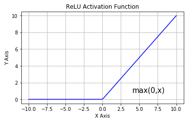
\[\begin{aligned} \phi(v)&=\tanh(v)\\ &=\frac{\exp(2v)-1}{\exp(2v)+1}\in(-1,1) \end{aligned}\]

Rectified Linear Unit (ReLU)

ReLU function graph ²

Most common choice in state-of-the-art neural networks (deep learning):

\[\phi(v)=\max(v,0)=\begin{cases}v&v\geq0\\0&v<0\end{cases}\]

Non-linear
Variants include leaky ReLU:
- Has a shallow negative gradient when $v<0$.

Network Architectures

Single-layer Feed-forward Network

One input layer of source nodes that project directly onto the output computation.

There are no cycles allowed.

The output can be calculated using the following function:

\[y_k(\mathbf X)=\phi\left(\sum^p_{j=0}W_{kj}X_j\right)\]

Multi-layer Feed-forward Network

⁴

Has additional hidden layers in-between the input and output. These provide a more capable network:

Typically the neurons of each layer take the previous layer as their input.
Still no cycles.

The output can be calculated using the following function:

\[y_k(\mathbf X)=\phi\left(\sum^{p_\text{hidden}}_{j=0}W_{kj}\underbrace{\phi\left(\sum^{p_\text{input}}_{i=0}W_{ji}\overbrace{X_i}^\text{input layer}\right)}_\text{hidden layer output}\right)\]

Convolutional Neural Networks (CNNs)

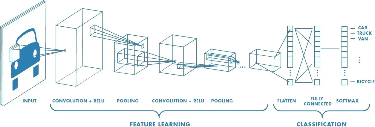
convoultional neural network processing an image ⁵

A class of multi-layer feed-forward network with a special type of local connections:

Widely used for image classification.
A convolution is used to gain deeper understanding of the image.

Recurrent Networks

These have feedback loops which form cycles in the graph:

Feedback loops involve connections with unit-delay elements $z^{-1}$, which together with nonlinear activations enable the nonlinear dynamic behaviour of the network.

We can calculate the output of a recurrent, no hidden, delay one, self feedback network with the following:

\[y_k(n)\equiv y_k(\mathbf X(n),n)=\phi\left(\underbrace{\sum^{p_\text{input}}_{i=0}W_{ki}X_i(n)}_\text{current input}+\underbrace{\sum^{p_\text{output}}_{j=0}W_{kj}y_j(n-1)}_\text{past output}\right)\]

Knowledge Representation

The primary task of a NN is to learn it’s environment. To accomplish this, we need to feed it with environment knowledge, which is based on:

Observations - These are often noisy, contain errors and have redundant/missing information.
- These can be labelled or unlabelled with the ground truth for that sample.

Training Dataset Example

A set ${{x_i, y_i}}, i=1,2,\ldots$ of experimentally acquired data is referred as a training dataset:

OCR:
- $x$ = Pixel values or curves.
- $y$ = A, B, C, …

Training Process

Choose a subset of the available observations as a training dataset to teach the NN.

This set should be diverse and representative of data used in production.
Choose an appropriate architecture, with as many input nodes as the length of the input feature vector $x$ and output nodes needed for the output $y$.
Train the network on the training dataset.
Test the network with the remaining data.