- Agent
- An agent is a computer system that is situated in some environment, and that is capable of autonomous action in that environment in order to meet its delegated objectives.
Agents can make their own decisions. Tele-operated systems aren’t agents.
Mobile Robotics
There are three main questions in mobile robotics:
- Where am I?
- Is there some sort of homing action?
- What is the target?
- How do I get there?
Types of Agents
Agents are on a scale of autonomy:
- Simple agents - Daemons, thermostats.
Agents vs Objects
| Agent |
Object |
| Agents are autonomous. |
Objects do it because they have to. |
| Agents are smart (proactive, reactive, social). |
Objects only act on request. |
| Agents act because they get a reward. |
|
Intelligent Agents
Intelligent agents exhibit three types of behaviour:
- Reactive (environment aware)
- Pro-active (goal-driven)
- Social Ability
Proactiveness
This is the act of generating and attempting to achieve goals, not solely by events.
This also includes recognising opportunities to achieve it’s goals.
Reactivity
If a program’s environment is fixed then it can act deterministically. We can react to changes in the environment.
Social Ability
This is the ability in agents to interact with other agents via cooperation, coordination and negotiation.
The basis of this is communication.
- Cooperation
- Working together as a team to achieve a goal.
- Coordination
- Managing the interdependences between activities (what should be done in what order).
- Negotiation
- The ability to reach agreements on matters of common interest.
Typically involves offer and counter-offer, with compromises made by participants.
Other Properties
- Mobility
- The ability for agents to move around a non-deterministic environment.
- Rationality
- Whether an agent will act in order to achieve it’s goals.
- Veracity
- Whether an agent will knowingly communicate false information.
- Benevolence
- Whether agents have conflicting goals or are working together.
- Learning/Adaptation
- Whether agents improve performance over time.
Agents With State
graph TB
Environment --> see
subgraph Agent
see --> next
next --> state
state --> next
state --> action
end
action --> Environment
Tasks for Agents
We want to tell agents to complete a particular task without telling them how to do it. We can achieve this with the following tools.
Utility Functions
- We associate rewards with states that we want agents to bring about.
- We associate utilities with individual states:
- The task of the agent is to bring about states that maximise utility.
A task specification is a function which associates a real number with every environment sate:
\[u:E\rightarrow\Bbb R\]
Local Utility Functions
How to we apply a utility score to a state in a run?
It is difficult to specify a long term view when assigning utilities to individual states.
One option would be to discount the cost for later states. This is what happens in reinforcement learning.
Local Utility Function Example
Consider we have a robot that wants to reach a reward:
- Each movement has a negative reward ($r=-0.04$)
- This ensures that the agent will learn to get the reward in the shortest path.
- The target has a positive reward ($r=1$)
The utility gained is the sum of the rewards received.
Mobile Robotics
To enable the robot to reach it’s goal then we need to consider the following:
- Locomotion & Kinematics
- Perception
- Localisation & Mapping
- Planning & Navigation
General Control Architecture
graph TB
l[Localisation/Map Building] -->|Position, Global Map| c[Cognition, Path Planning]
c -->|Path| pe[Path Execution]
subgraph Motion Control
pe -->|Actuator Commands| Action
end
Action -->|Real World, Environment| Sensing
subgraph Perception
Sensing -->|Raw Data| ie[Information Extraction]
end
ie -->|Environment Model, Local Map| l
Perception & Localisation
This is how the robot senses the world:
- A map then says how these features sit relative to one another.
- A robot localises by identifying features and the position in the map from which it could see them.
Navigation
This is the process for finding a path through the map:
- It is important that we avoid obstacles.
Architecture Approaches
Classical/Deliberative
Complete modelling:
- Function Based
- Horizontal Decomposition
graph LR
Sensors --> Perception
Perception --> lm[Localisation/Map Building]
lm --> cp[Cognition/Planning]
cp --> mc[Motion Control]
mc --> Actuators
Behaviour Based
- Sparse or no modelling.
- Behaviour Based
- Vertical Decomposition
- Bottom Up
graph LR
Sensors --> cd[Communicate Data]
Sensors --> da[Discover New Area]
Sensors --> dg[Detect Goal Position]
Sensors --> ao[Avoid Obsticals]
Sensors --> fw[Follow Right/Left Wall]
cd --> cf[Coordination Fusion]
da --> cf[Coordination Fusion]
dg --> cf[Coordination Fusion]
ao --> cf[Coordination Fusion]
fw --> cf[Coordination Fusion]
cf --> Actuators
Hybrid
This is a combination of the previous two approaches:
- Let lower level pieces be behaviour based:
- Localisation
- Obstacle avoidance
- Data collection
- Let more cognitive pieces be deliberative:
Reactive Architectures
Deliberative architectures aren’t always ideal as planning may take too long and the environment may have changed.
Brooks Behavioural Languages
- Intelligent behaviour can be generated without explicit representations of the kind that symbolic AI proposes.
- Intelligent behaviour can be generated without explicit abstract reasoning of the kind that symbolic AI proposes.
- Intelligence is an emergent property of certain complex systems.
He identified two key ideas that have informed his research:
- Situatedness and embodiment: ‘Real’ intelligence is situated in the world, not in disembodied systems such as theorem provers or expert systems.
- Intelligence and emergence: ‘Intelligent’ behaviour arises as a result of an agent’s interaction with its environment. Also, intelligence is ‘in the eye of the beholder’; it is not an innate, isolated property.
Emergent Behaviour
When observed behaviour exceeds the programmed behaviour, then we have emergence.
Flocking is an emergent behaviour. Each agent uses the following rules:
- Don’t run into any other agent.
- Don’t get too far from other agents.
- Keep moving if you can.
Synergies
We can implement the following behaviours to follow a wall:
- Move forwards with a slight bias towards the wall.
- Avoid obsticles by turning in the opposite direction.
This is the process of using simple rules to create complex behaviours.
Steel’s Mars Explorer System
Consider that we have a robot that we want to explore a distant planet and collect samples of rock. We know that the locations of the rocks tend to be clustered.
We can use the following rules from lowest to highest priority:
- If true, move randomly.
- If detect a sample then pick the sample up.
-
If carrying a sample and not at the base, then travel up gradient.
The gradient is a radio signal emitted by the mother-ship.
- If carrying a sample and at the base, then drop the sample.
- If detect an obstacle, then change direction.
Stigmergy
This is a act of communicating by leaving signs in the environment.
We can include this behaviour in our system to allow multiple agents to communicate and locate clusters of rock:
3. If carrying sample and not at the base, then drop 2 crumbs and travel up the gradient.
4.5. If sense crumbs, then pick up one crumb and travel down the gradient.
A crumb is a detectable piece of radioactive material.
Potential Fields
The robot is treated as a point under the influence of an artificial potential field.
- The filed depends on the targets and goal as well as desired travel directions.
- The goal attracts it, whilst obstacles repel it.
- The strength of the field may change with the distance to the obstacle or target.
The robot travels along the derivative of the potential.
This is similar to a ball rolling down a smooth surface.
Types of Fields
-
Uniform - guides the robot in a straight line

-
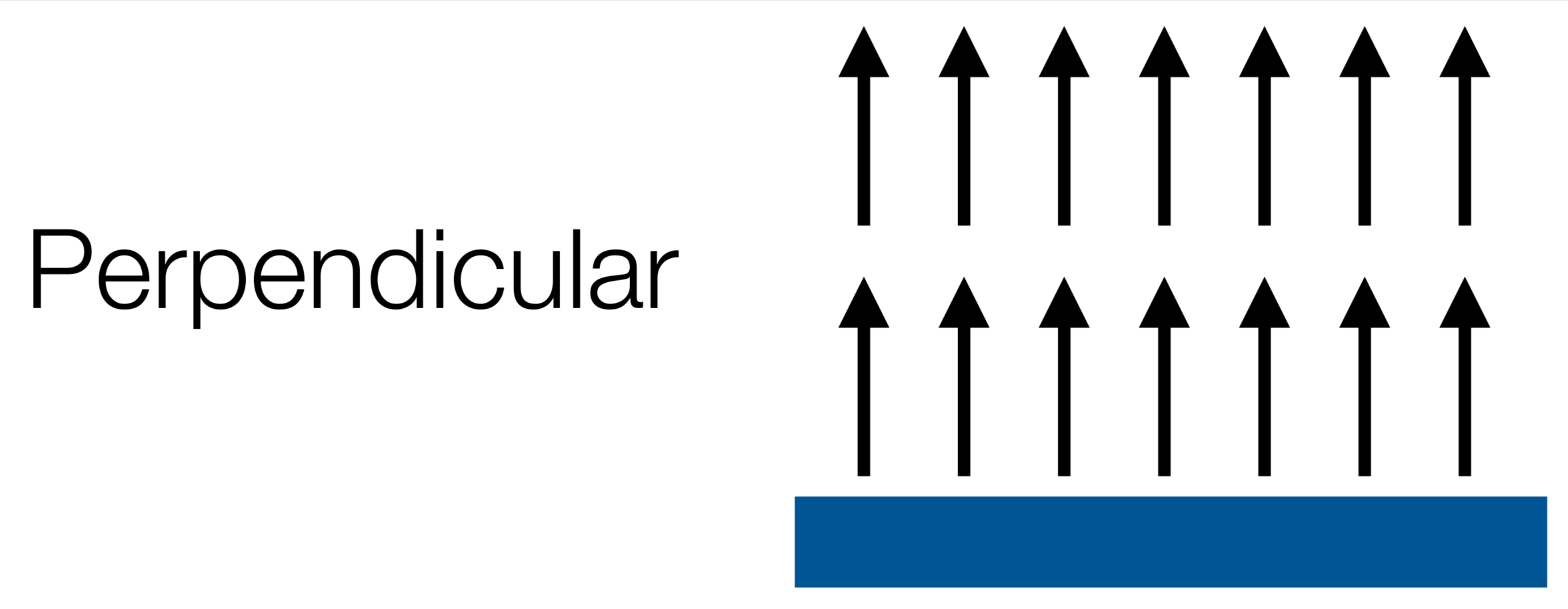
Perpendicular - pushes the robot away from linear obstacles

-
Tangential - guides the robot around an obsticle

-
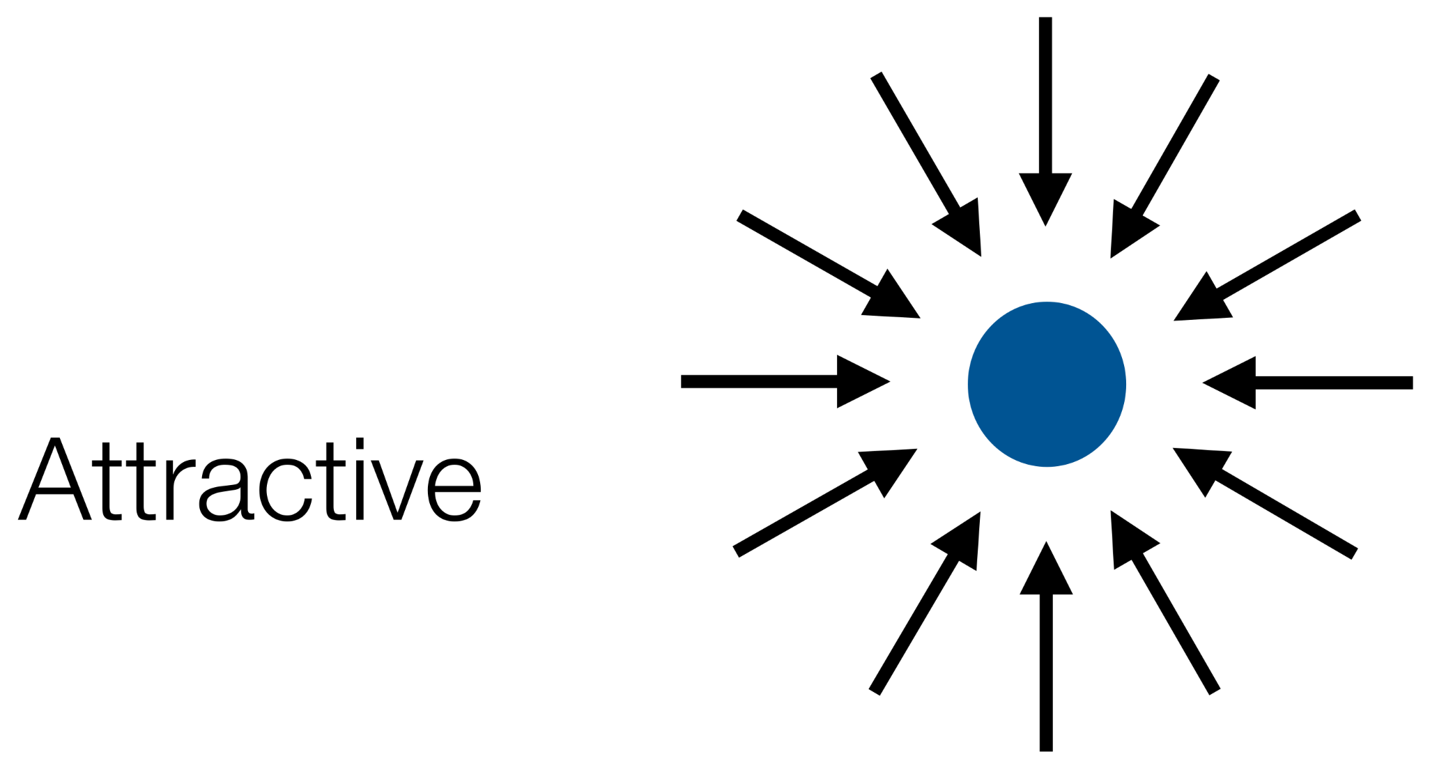
Attractive - draws the robot to a point

This can be useful for defining waypoints in a path.
-
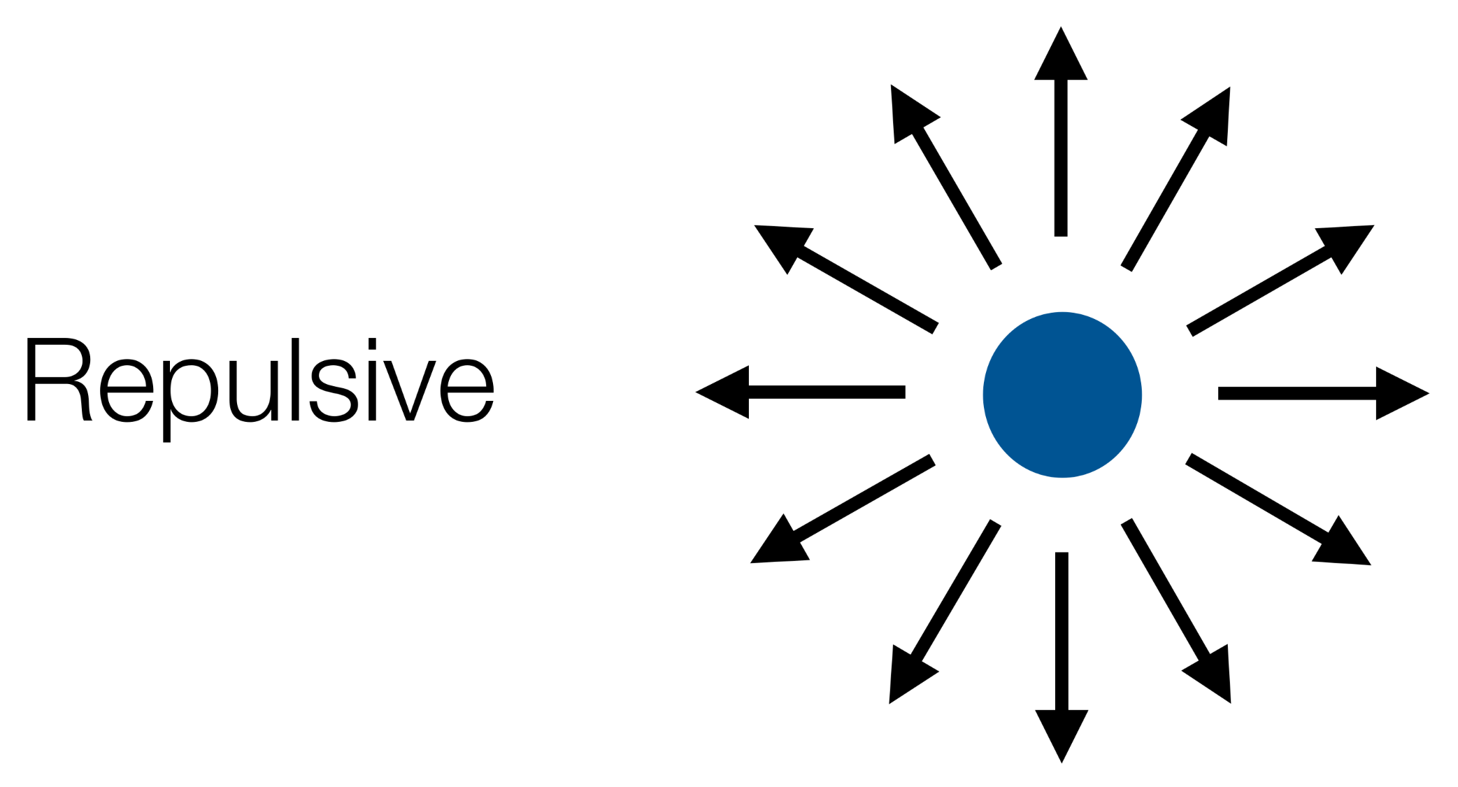
Repulsive - pushes the robot away from a point

Local Minima
One issue with potential fields is local minima. This is a well in the field.
There are various escape options:
- Backtracking
- Random Motioon
- Planner to search for a sub-optimal plan to escape.
- Increase potential of visited regions.
Characteristics of Potential Fields
Advantages:
- Easy to visualise.
- Easy to combine different fields.
Disadvantages:
- High update rates necessary.
- Parameter tuning is important.
Hybrid Architectures
Hybrid architectures combine both deliberative and reactive systems in order to control a robot.
In such an architectures, an agents control subsystems are arranged into a hierachy with higher layers dealing with information at increasing levels of abstraction.
Horizontal Layers
- Layers are each directly connected to the sensory input and action output.
- Each layer acts like an agent, producing suggestions as to what action to perform.
graph LR

pi[Perceptual Input] --> l1[Layer 1]
pi[Perceptual Input] --> l2[Layer 2]
pi[Perceptual Input] --> l3[Layer 3]
pi[Perceptual Input] --> ln[Layer n]
l1 --> ao[Action Output]
l2 --> ao[Action Output]
l3 --> ao[Action Output]
ln --> ao[Action Output]
Vertical Layering
Sensory input and action output are each dealt with by at most one layer each.
-
Vertical Layering (one pass control):
  graph LR
  pi[Perceptual Input] --> l1[Layer 1]
  l1 --> l2[Layer 2]
  l2 --> l3[Layer 3]
  l3 --> ln[Layer n]
  ln --> ao[Action Output]
-
Vertical Layering (two pass control):
  graph LR
  pi[Perceptual Input] -->|1| l1[Layer 1]
  l1 -->|2| l2[Layer 2]
  l2 -->|3| l3[Layer 3]
  l3 -->|4| ln[Layer n]
  ln -->|5| l3
  l3 -->|6| l2
  l2 -->|7| l1
  l1 -->|8| ao[Action Output]
Ferguson - TouringMachines
The TouringMachine architecture consists of perception and action subsystems:
- These interface directly with the agent’s environment, and three control layers, embedded in a control framework, which mediates between the layers.
graph LR
si[Sensor Input] --> pss[Perceptual Sub-System]
pss --> ml[Modelling Layer]
pss --> pl[Planning Layer]
pss --> rl[Reactive Layer]
subgraph Control Sub-System
ml
pl
rl
end
ml --> as[Action Subsystem]
pl --> as
rl --> as
as --> Actions
The control sub-system mediates between the layers.
- The reactive layer is implemented as a set of situation-action rules (like a subsumption architecture).
- The planning layer constructs plans and selects actions to execute in order to achieve the agents goals
- The modelling layer contains symbolic representations of the cognitive state of other entities in the agent’s environment.
Four Basic Wheel Types
- Standard Wheel
- Spherical Wheel - A ball with omnidirectional movement.
- Castor Wheel - A wheel that can rotate around a castor and it’s own axle.
- Swedish Wheel - A wheel made of 45 degree rollers. This allows passive motion in the direction of the rollers.
Characteristics of Wheeled Vehicles
- Stability is guaranteed with 3 wheels
- This is improved by using 4 or more wheels.
- Bigger wheels allow the robot to overcome higher obstacles.
- Most wheel arrangements are non-holonomic
- There are constraints in the direction that the vehicle can move.
- Combining actuation and steering on one wheel complicates design and adds odometry errors.
Locomotion of Wheeled Robots
The velocity of a wheel is determined by the wheel diameter and the change in rotation over time ($\omega=\frac{\Delta\theta}{\Delta t}$)
\[v = \omega r\]
This is an ideal scenario where there are no losses or deformation.
Wheels have two degrees of freedom. They can rotate in the x-axis and translate in the y-axis.
Mobility
The manoeuvrability of a vehicle depends on the degree of mobility:
- $\delta_m$ quantifies the degrees of controllable freedom based on changes to the wheel’s velocity.
\[\delta_m = 3 - N_k\]
where $N_k$ is the number independent kinematic constraints.
Independent means that they are on different axes.
$\delta_m$ quantifies the degrees of controllable freedom based on changes in wheel velocity.
Trike Degree of Mobility
A tricycle has:
- Two wheels in the same axis as the back.
- Even if they can turn independently they are on the same axis, therefore dependant.
- A front steering wheel.
This gives two kinematic constraints therefore the degree of mobility is:
\[\delta_m = 3 - 2 = 1\]
Steerablity
The degree of steerability ($\delta_s$) is the number of independent steerable wheels (where $0\leq\delta_s\leq2$).
$\delta_s$ quantifies the degrees of controllable freedom based on changes in wheel orientation.
Manoverability
- The degree of manoeuvrability $\delta_M$
- The overall degrees of freedom that a robot can manipulate by changing the wheel’s speed and orientation
\[\delta_M = \delta_m+\delta_s\]
This is an indicator as to how easy it is for a robot to move around.
Non-Holonomic Constraints
Vehicles with non-holonomic constraints are unable to move in all directions of a 2D plane:
- A Bike has non-holonomic contraints as it has to rotate in order to go left or right.
- A ball is holonomic as it can move in any direction.
Instantaneous Center of Rotation
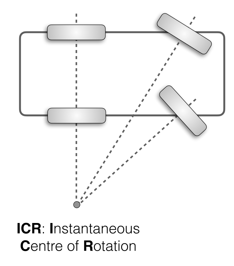
In a connected drive system (like a car), all wheels have to move along a circle.
If travelling forward, the circle is infinely large.
The centre of this turning circle is the convergence of all of the axels. This point is the ICR (Instantaneous Centre of Rotation)

Differential Drive
- $R$
- This is the radius of the current turning circle of the robot. The radius of the ICR.
- $\omega$
- This is the rotational velocity, about the ICR, of the robot $\omega=\frac{\Delta \theta}{\Delta t}$.
- $l$
- The distance between the wheels of the robot.
Forward Velocity of the Robot
\[\begin{aligned}
v &= \omega R\\
v &= \frac{v_r+v_l} 2
\end{aligned}\]
Velocities of the Wheels
\[\begin{aligned}
v_l&=\omega(R-\frac l 2)\\
v_r&=\omega(R+\frac l 2)\\
\end{aligned}\]
ICR Radius
\[R=\frac l 2\times \frac{v_l+v_r}{v_r-v_l}\]
Rotational Velocity
\[\omega = \frac{v_r-v_l} l\]
If the wheel velocities are equal then $\omega = 0$ and the robot moves forward.
Rotation Matrix
A rotation matrix is used to perform a rotation in Euclidean space. The following function rotates counter-clockwise through angle $\theta$ around the origin:
\[R(\omega)=
\begin{bmatrix}
\cos(\theta) & -\sin(\theta)\\
\sin(\theta) & \cos(\theta)
\end{bmatrix}\]
We can use this to rotate a coordinate as a vector:
\[\begin{aligned}
\begin{bmatrix}
x'\\y'
\end{bmatrix} =&
\begin{bmatrix}
\cos(\theta) & -\sin(\theta)\\
\sin(\theta) & \cos(\theta)
\end{bmatrix}
\begin{bmatrix}
x\\y
\end{bmatrix}\\
=&
\begin{bmatrix}
x\cos(\theta) & -y\sin(\theta)\\
x\sin(\theta) & y\cos(\theta)
\end{bmatrix}
\end{aligned}\]
Differential Drive - Kinematics
To determine where the robot is, given an angular momentum $\omega$ after $\delta t$, wie can use the rotation matrix:
- Translate the ICR to the origin (subtract the coordinates of the ICR from the robot position $(x,y)$).
- Apply the rotation matrix.
- Reposition the final location, taking into account the original ICR location.
- Add the angular distance $\omega\delta t$ to the robot’s orientation.
\[\begin{bmatrix}
x'\\y'\\\theta'
\end{bmatrix}=
\underbrace{\begin{bmatrix}
\cos(\omega\delta t)&-\sin(\omega\delta t)&0\\
\sin(\omega\delta t)&-\cos(\omega\delta t)&0\\
0&0&1
\end{bmatrix}}_\text{Step 2}
\underbrace{\begin{bmatrix}
x - \text{ICR}_x\\
y - \text{ICR}_y\\
\theta
\end{bmatrix}}_\text{Step 1}+
\underbrace{\begin{bmatrix}
\text{ICR}_x\\
\text{ICR}_y\\
\omega\delta t
\end{bmatrix}}_\text{Steps 3 and 4}\]
Random Variables
Discrete Random Variables
A set $X$ which contains a finite number of values ${x_1,x_2,\ldots,x_n}$
$P(X=x_i)$ (or $P(x_i)$) is the probability that the random variable $X$ takes on the value $x_i$.
Continuous Random Variables
$X$ takes on values along a bell curve.
$p(X=x)$ (or $p(x)$) is a probability density function
A probability density function would look like so:
\[P(x\in(a,b)) = \int^b_ap(x)dx\]
This will be approximated by splitting the range into discrete values.
Joint and Conditional Probability
Joint Probability
If $X$ and $Y$ are independent:
\[P(x,y) = P(x)P(y)\]
Conditional Probability
Probability of $x$ given $y$:
\[P(x\mid y)=\frac{P(x,y)}{P(y)}\]
given that $x$ and $y$ are conditional:
\[P(x,y) = P(x\mid y)P(y)\]
If $x$ are $y$ are independent:
\[\begin{aligned}
P(x\mid y)&=\frac{P(x,y)}{P(y)}\\
&=\frac{P(x)P(y)}{P(y)}\\
&=P(x)
\end{aligned}\]
Theorem of Total Probability & Marginals
Marginalisation
-
Discrete Case
\[P(x)=\sum_yP(x,y)\]
-
Continuous Case
\[p(x)=\int p(x,y)dy\]
Theorem of Total Probability
This follows from marginalisation as $P(x,y)=P(x\mid y)P(y)$:
-
Discrete Case
\[P(x)=\sum_yP(x\mid y)P(y)\]
-
Continuous Case
\[p(x)=\int p(x\mid y)p(y)dy\]
The joint probability of $x$ and $y$ is commutative:
\[P(x.y) = P(x\mid y)P(y) = P(y\mid x)P(x)\]
From this we can derive the Bayes Formula:
\[P(x\mid y) = \frac{P(y\mid x)P(x)}{P(y)}\]
\[\text{posterior} = \frac{\text{likelihood}\times\text{prior}}{\text{evidence}}\]
Normalisation
As $P(y)$ doesn’t depend on $x$ then we can replace it with a normaliser ($\eta=P(y)^{-1}$):
\[\begin{aligned}
P(x\mid y) &= \frac{P(y\mid x)P(x)}{P(y)}\\
&=\eta P(y\mid x)P(x)
\end{aligned}\]
We can then calculate $\eta$ at a later stage:
\[\eta=\frac 1{\sum_xP(y\mid x)p(x)}\]
Bayes Rule with Background Knowledge
Consider we want to calculate the probability of $x$ given $y$ and $z$. We can write this as:
\[P(x\mid y,z) = \frac{P(y\mid x,z)P(x\mid z)}{P(y\mid z)}\]
State Estimation
Consider that we want to determine whether a door is open or closed:
- A robot obtains measurement $z$ from its sensor
We need to determine:
\[P(\text{open}\mid z)\]
Diagnostic vs. Causal
We can use causal knowledge to generate diagnostic knowledge by using Bayes:
\[P(\text{open}\mid z)=\frac{P(z\mid\text{open})P(\text{open})}{P(z)}\]
Probability Distribution Function
Assume we measure a number of sensor samples:
- When the door was closed.
- When the door was open.
This gives us the probability distribution function (PDF) for some sensor when the door is open.
In this example we can assume:
- $P(z\mid \text{open}) = 0.6$
- $P(z\mid\neg\text{open})=0.3$
As we don’t know if the door is open or not, we assume uniform distribution for the prior:
\[P(\text{open})=P(\neg\text{open})=0.5\]
State Estimation Example
Given that:
- $P(z\mid\text{open})=0.6$
- $P(z\mid\neg\text{open})=0.3$
- $P(\text{open})=P(\neg\text{open}) =0.5$
We have:
\[\begin{aligned}
P(\text{open}\mid z)&=\frac{P(z\mid\text{open})P(\text{open})}{P(z\mid\text{open})P(\text{open})+P(z\mid\neg\text{open})P(\neg\text{open})}\\
&=\frac{0.6\times0.5}{(0.6\times0.5)+(0.3\times0.5)}\\
&=0.67
\end{aligned}\]
Recursive Bayesian Updating
Suppose we have additional sensors ($z_1,\ldots,z_n$) we want to inform our estimation with. We want to estimate:
\[P(x\mid z_1,\ldots,z_n)\]
We can estimate $x$ given observations $z_1,\ldots,z_n$:
\[P(x\mid z_1,\ldots,z_n) = \frac{P(z_n\mid x,z_1,\ldots,z_{n-1})P(x\mid z_1,\ldots,z_{n-1})}{P(z_n\mid z_1,\ldots,z_{n-1})}\]
To simplify this:
- We have the recursive term $P(x\mid z_1,\ldots,z_{n-1}$ in the numerator.
- We also know we can handle the denominator with normalisation.
- We can use the Markov assumption on the term $P(z_n\mid x, z_1,\ldots,z_{n-1})$:
- This term refers to the likelihood of a measurement givent that I know what the state of the door is ($x$) and I know all my previous measurements.
- If we only have the priors $z_1,\ldots,z_{n-1}$ then $z_n$ woudl be depentent by the priors.
- However, we know the current state $x$, so $z_n$ is independent
of $z_1,\ldots,z_{n-1}$. Hence the Markov assumption.
Maximum a Posteriori Estimation
This simplification is called maximum a posteriori estimation and it is written like so:
\[\begin{align}
P(x\mid z_1,\ldots,z_n) &= \frac{P(z_n\mid x,z_1,\ldots,z_{n-1})P(x\mid z_1,\ldots,z_{n-1})}{P(z_n\mid z_1,\ldots,z_{n-1})}\\
&=\frac{P(z_n\mid x)P(x\mid z_1,\ldots,z_{n-1})}{P(z_n\mid z_1,\ldots,z_{n-1})}\tag{Markov Assumption}\\
&=\eta P(z_n\mid x)P(x\mid z_1,\ldots,z_{n-1})\tag{Normalisation}\\
&=\eta_{1\ldots n}\left[\prod_{i=1\ldots n}P(z_i\mid x)\right]P(x)\tag{Recursive Term}
\end{align}\]
State Estimation with Multiple Sensors Example
Given that:
- $P(z\mid\text{open})=0.6$
- $P(z\mid\neg\text{open})=0.3$
- $P(\text{open})=P(\neg\text{open}) =0.5$
- $P(\text{open}\mid z_1) = 0.67$
- $P(\neg\text{open}\mid z_1) = 1-P(\text{open}\mid z_1) = 0.33$
- $P(z_2\mid \text{open}) = 0.5$
- $P(z_2\mid\neg\text{open}) = 0.6$
We have:
\[\begin{aligned}
P(\text{open}\mid z_2,z_1) &= \frac{P(z_2\mid\text{open})P(\text{open}\mid z_1)}{P(z_2\mid\text{open})P(\text{open}\mid z_1)+P(z_2\mid\neg\text{open})P(\neg\text{open}\mid z_1)}\\
&=\frac{\frac12\times\frac23}{(\frac12\times\frac23)+(\frac35\times\frac13)}\\
&=\frac58=0.625
\end{aligned}\]
Modelling Actions
Actions are never carried out with absolute certainty.
To incorporate the outcome of an action $u$ into the current belief, we use the conditional PDF $P(x\mid u,x’)$:
- This term specified the PDF that executing action $u$ changes the state from $x’$ to $x$.
Generating a PDF for Actions
The probability distribution function can be generated by:
- Placing the robot in some state $x’$.
- Executing the action $u$.
- Measuring the state $x$.
These steps are then repeated a large number of times to build the PDF for the action $u$.
Modelling Action Example
Assume we have the PDF $P(x\mid u,x’)$ for the action $u=\text{close door}$. This can be represented as an FSM:
stateDiagram-v2
direction LR
open --> closed:0.9
closed --> closed:1
closed --> open:0
open --> open:0.1
We can read: if the door is open, the action “close door” succeeds in 90% of all classes.
Integrating the Outcome of Actions
To find $P(x\mid u)$ we sum (or integrate) over all the possible prior states (values of $x’$).
-
Continuous case:
\[P(x\mid u)=\int P(x\mid u,x')P(x'\mid u)dx'\]
-
Discrete case:
\[P(x\mid u)=\sum_{x'}P(x\mid u,x')P(x'\mid u)\]
We can assume that the action $u$ tells us nothing about the prior state of the door, and can be removed:
-
Continuous case:
\[P(x\mid u)=\int P(x\mid u,x')P(x')dx'\]
-
Discrete case:
\[P(x\mid u)=\sum_{x'}P(x\mid u,x')P(x')\]
Calculating Belief Example
Given the following FSM and our sensor samples:
stateDiagram-v2
direction LR
open --> closed:0.9
closed --> closed:1
closed --> open:0
open --> open:0.1
- $P(\text{open}) = \frac58$
- $P(\text{closed}) = \frac38$
We can calculate:
\[\begin{align}
P(\text{closed}\mid u) &= \sum_{x'}P(\text{closed}\mid u,x')P(x')\\
&= P(\text{closed}\mid u,\text{open}) + P(\text{closed}\mid u,\text{closed})P(\text{closed})\\
&=\left(\frac9{10}\times\frac58\right)+\left(\frac11\times\frac38\right)\\
&=\frac{15}{16}
\end{align}\]
\[\begin{align}
P(\text{open}\mid u) &= \sum_{x'}P(\text{open}\mid u,x')P(x')\\
&=P(\text{open}\mid u,\text{open})P(\text{open})+P(\text{open}\mid u,\text{closed})P(\text{closed})\\
&=\left(\frac1{10}\times\frac58\right)+\left(\frac01\times\frac38\right)\\
&=\frac1{16}=1-P(\text{closed}\mid u)
\end{align}\]
Bayes Filters
Bayes filters allow us to:
- Calculate the posterior of the current state, the belief:
- $\text{Bel}(x_t)=P(x_t\mid u_1, z_1,\ldots,u_t,z_t)$
$t$ is the current time.
To do this we need the following information:
Calculating Belief
Belief ca be derived as:
\[\text{Bel}(x_t)=\eta P(z_t\mid x_t)\int P(x_t\mid u_t,x_{t-1})\text{Bel}(x_{t-1})dx_{t-1}\]
this reduces to the following sum:
\[\text{Bel}'(x)=\sum P(x\mid u,x')\text{Bel}(x')\]
Typical Motion Models
Typically there are two types of motion model:
- Odometry-based
- Used when systems are equipped with proprioceptive sensors such as wheel encoders.
- Velocity-based (Dead reckoning)
- Used based purely on velocities and time elapsed, using no sensors.
Classification of Sensors
Proprioceptive Sensors
Measure values internally, measuring direct feedback on the robot. This can include:
- Wheel Encoders
- Motor Load
Exteroceptive Sensors
Measure values from the environment. These can be:
- Ambient light sensors
- Radar
Passive Sensors
Measure energy from the environment, have no external effect. They can include:
- Accelerometers
- Thermometers
Active Sensors
Emit their own energy and measure the reaction. These include:
Coping with Errors
In general odometry doesn’t hold up well over long distances:
- Range Error
- Integrated path length (distance) of the robots movement.
Sum of the wheel movements.
- Drift Error
- Difference in the error of the wheels leads to an error in the robot’s angular orientation.
- Turn Error
- Similar to range error, but for turns.
Difference of the wheel motions.
Over long periods of time, turn and drift errors far outweigh range errors.
Relative Odometry
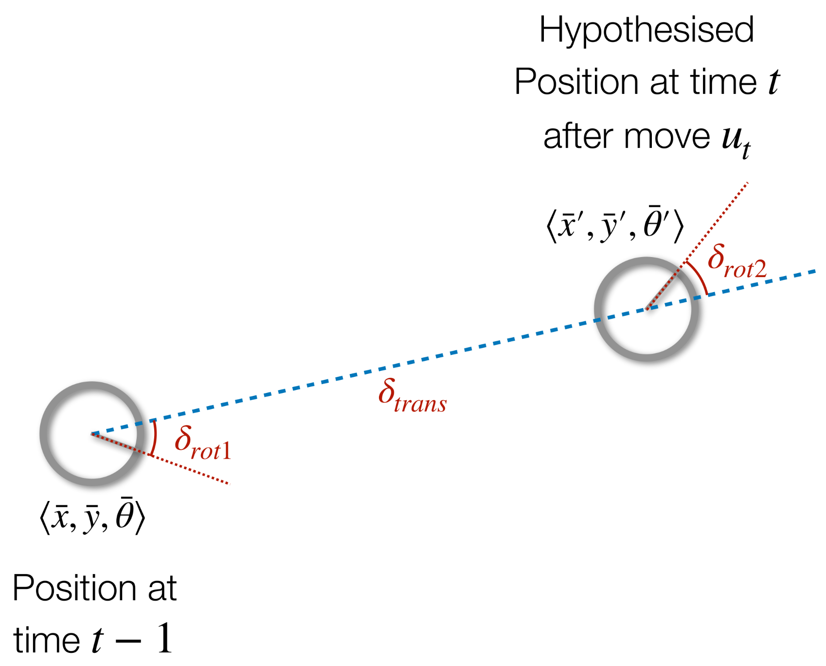
We can encode a position like so:
\[\langle x,y,\theta\rangle\]
Where $x$ and $y$ are the Cartesian coordinates and $\theta$ is the direction the robot is facing:

We can write our believed position as $\langle \bar x,\bar y,\bar\theta\rangle$. This is opposed to the true location which is written as $\langle \hat x,\hat y,\hat\theta\rangle$
Odometry is the difference between two poses:
\[u=\langle\delta_\text{rot1},\delta_\text{trans},\delta_{rot2}\rangle\]
where:
\[\begin{align}
\delta_\text{rot1}&=\text{atan2} (y'-y,x'-x)-\theta\\
\delta_\text{trans}&=\sqrt{(x-x')^2+(y-y')^2}\\
\delta_\text{rot2}&=\theta'-\theta-\delta_\text{rot1}
\end{align}\]
$\text{atan2}$ is defined as so:
\[\text{atan2}(y,x) = \begin{cases}
\arctan(\frac yx)&\text{if }x>0\\
\text{sign}(y)(\pi-\arctan(\lvert \frac yx\rvert))&\text{if }x<0\\
0&\text{if }x=y=0\\
\text{sign}(y)\frac\pi2&\text{if }x=0,y\neq0
\end{cases}\]
Odometry Model
What is the likelihood that $u_t$ took us from $\bar x_{t-1}$ to $\bar x_t$?
Where $\bar x_{t-1}$ and $x_t$ are our believed location before and after respectively.
We can determine the true odometry $\hat u_t$ via a model:
- We are trying to determine $p(\hat u_t\mid u_t)$ which can be solved by determining $p(x_t\mid u_t,x_{t-1})$, where:
- new location/state: $\text{pose}(x_t)$
- the motion/action: $\text{odometry}(u_t)$
- original location/state: $\text{pose}(x_{t-1})$
Model for Odometry with Noise
To calculate the true motion we should account for independent noise. We can do this using six coefficients $\alpha_1,\ldots,\alpha_6$. These can be calculated using sampling.
Noisy Initial Rotation
\[\hat\delta_\text{rot1} = \delta_\text{rot1}+\epsilon_{\alpha_1\lvert\delta_\text{rot1}\rvert+\alpha_2\lvert\delta_\text{trans}\rvert}\]
Note that we take the absolute value using $\lvert x\rvert$. This doesn’t mean given that.
where:
- $\alpha_1$ - possibly due to error on the inital rotation.
- $\alpha_2$ - possibly due to forces on the robot as it moves forward.
Noisy Translational Error
\[\hat\delta_\text{trans}=\delta_\text{trans}+\epsilon_{\alpha_3\lvert\delta_\text{trans}\rvert+\alpha_4\lvert\delta_\text{rot1}+\delta_\text{rot2}\rvert}\]
where:
- $\alpha_3$ - possibly due to error with the translation.
- $\alpha_4$ - initial and final rotation can result in a drift in position.
Noisy Final Rotation
\[\hat\delta_\text{rot2}=\delta_\text{rot2}+\epsilon_{\alpha_5\lvert\delta_\text{rot2}\rvert+\alpha_6\lvert\delta_\text{trans}\rvert}\]
where:
- $\alpha_5$ - possibly due to error on the final rotation.
- $\alpha_6$ - possibly due to the resulting translational movement that may further rotate the robot.
Many models assume that the initial and final rotations have similar characteristics and assume $\alpha_5=\alpha_1$ and $\alpha_6=\alpha_2$.
Modelling $\epsilon$
The distributions have a zero-centred mean, and $b=\sigma=\text{standard deviation}$.
Feedback Control
So far we have seen open loop control. This is where we make an observation, determine a plan to reach the goal and then execute that plan:
- This doesn’t account for errors in the action of moving to the goal, or changes in the environment.
graph LR
input  --> ra[Robot Actuator] --> output
Closed Loop
This is where we sense the result of an action and feed back to adjust the action:
- A reference signal (set point) is sent to the control.
- The input is observed, resulting in a measured value.
- The difference between the set point and measure is the error.
- Error can then be converted into a control input.
graph LR
setpoint --> delta
output --> delta
delta -->|error| control
control -->|control input| ra[Robot Actuator]
ra --> output
The aim is to reduce the error to zero.
As a robot is a dynamic system the control should be a function of:
- Present Behaviour
- Past Behaviour
- Future Behaviour
Present Behaviour
This part of the controller focusses on current behaviour:
-
The output is proportional to the magnitude of the error:
\[o_p\propto K_p\]
where $K_p$ is the proportional gain for the proportional factor of the error.
This gain determines how much the current error affects any changes to the input.
Correcting an error may result in over-correction. This will produce an oscillation that should be dampened. This can be achieved by:
Future Behaviour
Momentum generated by a controllers response can cause oscillation:
- The control needs to be different when the system is close to the set point, compared to when it is far away.
This can be resolved by looking at future error:
-
This is the gradient, or differential, of $o_p$:
\[o_d=K_d\frac {de}{dt}\]
where $K_d$ is the derivative gain for the derivative factor oif the error.
We can generate $K_d$ by comparing current and past error rates:
\[o\approx K_d(e_t-e_{t-1})\]
The derivative opposes the velocity of the proportionate control.
Past Behaviour
Past error is tracked by the integral term:
It should be generated over time such that:
\[o_t=o_{t-1}+e_t\]
PID Controllers
A PID controller is the sum fo the proportional $p$, integral $i$ and derivative $d$ control terms:
\[o=K_pe+K_i\int e(t)dt+K_d\frac{de}{dt}\]
where the gains determine the significance of each of the terms.
flowchart RL
a(( )) -->|setpoint| b(( ))
b -->|error, e| control
subgraph control
direction LR
proportional
integral
derivative
end
proportional --> +((+))
integral --> +
derivative --> +
+ -->|control input, c| rc[robot control]
rc -->|output| c(( ))
rc --> b
If state errors are negligent then we can use a PD controller:
\[o=K_pe+K_d\frac{de}{dt}\]
Exteroceptive Sensors
This is a class of sensors that measure information about a robot’s external environment. They are characterised by a number of different attributes:
Field of View & Range
Every sensor has a region of space that it can cover:
- The width of that region is the field of view $\beta$
- The range $R$ is how far the field of view extends.
- Sensitivity
- Measure of the degree to which incremental changes in the target input change the output signal.
The ratio of output change to input change.
- Cross-sensitivity
- Sensitivity to environmental parameters that are orthogonal to the target parameters.
An example is that a compass is sensitive to magnetic north, but also to ferrous materials.
Accuracy & Precision
- Accuracy (Error)
- Difference between the sensor’s measured value, $m$ and the true value $v$, such that:
\[\begin{align}
\text{error}&=m-v\\
\text{accuracy}&=1-\frac{\lvert m-v\rvert}v
\end{align}\]
- Precision
- Reproducibility sensor results. If the random error of a sensor is characterised by some mean $\mu$ and standard deviation $\sigma$, the the precision is the ration of the sensors output range to $\sigma$.

Systematic & Random Error
Systematic errors are deterministic:
- Caused by factors that can be modelled and corrected.
Random errors are non-deterministic:
- No prediction is possible.
- They can be described probabilistically, like errors in wheel odometry.
Resolution, Linearity & Frequency
- Resolution
- The minimum difference between two values.
- Bandwidth (Frequency)
- The speed which which a sensor can provide readings.
Responsiveness
Most sensors work poorly in certain domains. Therefore we should use sensors that have a good signal-to-noise ratio in their application.
For example, sonar works poorly in environments with large amounts of glass due to the large amount of specular reflection.
Behavioural Sensor Function
- Sensor Fusion
- The combination of information from multiple sensors into a single percept.
We want to use multiple sensors for the following reasons:
- Redundancy
- Complementary - Difference percepts that support each-other.
- Touch sensors when objects are too close to be detected by sonar.
- Coordinated - Using one sensor as a consequence of a percept detected by another.
- Detecting a possible obstacle using a range sensor and verifying it’s existence using a tactile sensor.
| |
Observed Feature |
No Feature Observed |
| Feature Exists |
True Positive |
False Negative |
| Nothing to Perceive |
False Positive |
True Negative |
Sensor Fusion
Sensor fusion ca be combined with behaviours in different ways:
- Sensor Fission
- One sensor per behaviour.
- Behaviours can share sensor streams.
  graph LR
  s1[sensor] -->|percept| b1[behaviour] -->|action| cm[combination mechanism]
  s2[sensor] -->|percept| b2[behaviour] -->|action| cm[combination mechanism]
  s3[sensor] -->|percept| b3[behaviour] -->|action| cm[combination mechanism]
  cm -->|action| x(( ))
- Action-Oriented Sensor Fusion
- The combination of sensor data may trigger different different behaviours.
- An abstract percept emerges form the fusion of several percepts.
  graph LR
  s1[sensor] -->|percept| fusion
  s2[sensor] -->|percept| fusion
  s3[sensor] -->|percept| fusion
  fusion -->|percept| behaviour
  behaviour -->|action| x(( ))
Rejection Sampling
If we have a function $f$ we can sample random values from this function using the following method:
- Sample $x$ from a uniform distribution $[-b,b]$.
- Sample $y$ from $[0,\max f]$
- If $f(x)>y$ then keep the sample.
- Otherwise reject.
Sampling vs Odometry
- Sampling
- Determines a predicted new pose based on an initial pose $x_{t-1}$ and the motion $u_t$.
When sampled multiple times, a point cloud is gained, representing the probability distribution for possible end locations.
- Odometry
- Provides a closed form expression for generating the probability of being in a location. This is computing the posterior: $p(x_t\mid u_t,x_{t-1})$.
Map-Consistent Motion Model
We can rewrite the bayesian filter to include background knowledge of a map. The motion model becomes:
\[p(x_t\mid x_{t-1}, u_t, m)\]
graph LR
p((Past)) --> xt-1
xt-1 --> xt --> xt+1
ut-1 --> xt-1 --> zt-1
ut --> xt --> zt
ut+1 --> xt+1 --> zt+1
zt-1 --- m
zt --- m
zt+1 --- m
xt+1 --> a((future))
Knowlege about features like walls, change the resulting probabilities.
The aim of the sensor model is to determine:
\[P(z\mid x)\]
what is the probability of a measurement $z$, given that the robot is in state $x$.
Beam-Based Sensor Model
Consider each beam from the robot’s sensors independently. A scan $z$ is made up of $K$ measurements:
\[z=\{z_1, \ldots,z_K\}\]
Individual measurements are independent given the robot position:
\[P(z\mid x, m)=\prod^k_{k=1}P(z_k\mid x, m)\]
This assumes that we already have a map.
We may get the following types of erroneous readings:
- Measurement Noise
- Unexpected Obstacles
- Random Measurements
- Max Range
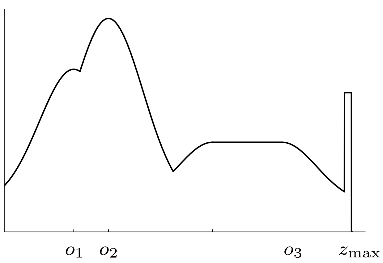
We can then combine these to form a combined distribution such that we can determine:
\[P(z\mid x,m)\]
This will be different depending on the type of erroneous reading.
Measurement Noise
We can calculate this as:
\[P_\text{hit}=\eta\frac1{\sqrt{2\pi b}}e^{-\frac12\frac{(z-z_\text{exp})^2}{b}}\]
Consider we calculate an expected sensor value $z_\text{exp}$. We can calculate:
\[p(z\mid z_\text{exp})\]
as the distribution is limited to $[0,z_\max]$, we normalise with:
\[\eta=\left(\int^{z_\max}_0\frac1{\sqrt{2\pi b}}e^{-\frac12\frac{(z-z_\text{exp})^2}{b}}dz^k_t\right)^{-1}\]
Unexpected Obstacles
We can model this with the following distribution:
\[P_\text{unexp}=\begin{cases}\eta\lambda e^{-\lambda z}&z<z_\text{exp}\\0&\text{otherwise}\end{cases}\]
where $\lambda>0$ is the rate paramter and $z$ is the query point.
As the exponential range is limited to $[0,z]$, we normalise with:
\[\eta=\frac1{1-e^{\lambda z}}\]
Max Range
We can model this with the following distribution:
\[P_\text{max}=\begin{cases}1&z=z_\max\\0&\text{otherwise}\end{cases}\]
Resulting Mixture Density
We can combine this by calculating the weighted sum of all the distributions:
\[P(z\mid x, m)=\begin{pmatrix}
\alpha_\text{hit}\\
\alpha_\text{unexp}\\
\alpha_\max\\
\alpha_\text{rand}
\end{pmatrix}^T\cdot
\begin{pmatrix}
P_\text{hit}(z\mid x, m)\\
P_\text{unexp}(z\mid x, m)\\
P_\text{max}(z\mid x, m)\\
P_\text{rand}(z\mid x, m)\\
\end{pmatrix}\]
Determining Intrinsic Values
The sensor model is tuned through a set of intrinsic values:
\[\Theta=\langle\alpha_\text{hit}, \alpha_\text{unexp}, \alpha_\max, \alpha_\text{rand}, \sigma, \lambda\rangle\]
This consists of the weights where:
\[\alpha_\text{hit}+ \alpha_\text{unexp}+ \alpha_\max+ \alpha_\text{rand}=1\]
and the distribution parameters:
- $\lambda$ for the exponential distribution
- The probability when $z=0$.
- $\sigma$ for the normal distribution
- The width of the Gaussian.
Beam Based Range Finder Algorithm
See slide 74 for this algorithm.
Refer to the slides, from 81-94 for this lecture as there are a lot of diagrams.
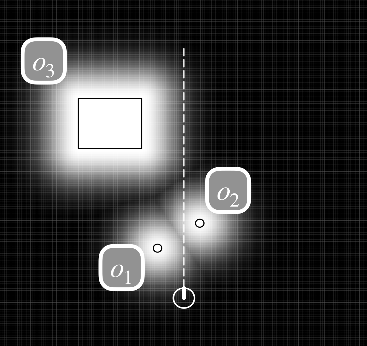
Consider we have a map with objects in it. We can make a likelihood field by applying a Gaussian distribution to the edge of each object in the map.


Modelling a Robot with 6 Sensors
- There is a worked example in the slides of calculating the pose of each sensor on a robot.
Finding the Location of Scan $z_t$
To find the location of a scan $z_t$ in global coordinate space:
Calculating the Likelihood Field
As with the beam model we combine the weighted sum of the three distributions:
For scan models, we omit unexpected obstacles.
-
Measurement Noise
\[P_\text{hit}=\eta\frac1{\sqrt{2\pi b}}e^{-\frac12\frac{(z-z_\text{exp})^2}{b}}\]
-
Random Measurements
\[P_\text{rand}=(z\mid x, m) = \begin{cases}
\frac1{z_\max}&\text{if }0\leq z\leq z_\max\\
0&\text{otherwise}
\end{cases}\]
-
Max Range
\[P_\text{max}=\begin{cases}1&z=z_\max\\0&\text{otherwise}\end{cases}\]
We can combine this by calculating the weighted sum of all the distributions:
\[P(z\mid x, m)=\begin{pmatrix}
\alpha_\text{hit}\\
\alpha_\max\\
\alpha_\text{rand}
\end{pmatrix}^T\cdot
\begin{pmatrix}
P_\text{hit}(z\mid x, m)\\
P_\text{max}(z\mid x, m)\\
P_\text{rand}(z\mid x, m)\\
\end{pmatrix}\]
where:
\[\alpha_\text{hit}+
\alpha_\max+
\alpha_\text{rand}=1\]
We can also use the following models to localise a robot:
- Map Matching (sonar, laser)
- Generate small, local maps from sensor data and match local maps against a global model.
- Scan Matching (laser)
- Map is represented by scan endpoints, match scan into this map.
- Beacons (sonar, laser, vision)
- Extract features such a doors hallways from sensor data.
Landmarks & Beacons
This is the process of localising using beacons. They can be of the following types:
This is different to previous sensor models as we are looking for specific landmarks:
- These observations can be used to estimate current location.
- The standard approach is to use triangulation or trilateration.
A sensor provides a combination of:
- Range $r$.
- Bearing $\phi$
- Signature $s$ which describes the feature:
Landmarks should be of the following type:
- Be readily recognisable
- Perceivable from many different viewpoints.
Landmarks
A feature vector represents an observed landmark. It is given as a collection of triples:
\[f(z_t=\{f^1_t,f^2_t,\ldots\}=\left\{
\begin{pmatrix}r^1_t\\\phi^1_t,\\s^1_t\end{pmatrix},
\begin{pmatrix}r^2_t\\\phi^2_t,\\s^2_t\end{pmatrix},
\ldots\right\}\]
By assuming conditional independence, we can consider one feature at a time such that:
\[p(f(z_t)\mid x_t, m)=\prod p(r^i_t, \phi^i_t, s^i_t\mid x_t, m)\]
We can combine this with map data in order to localise the robot.
A map is a list of objects and their locations:
\[m=\{m_1, m_2, \ldots,m_N\}\]
We are assuming that the map is feature based with landmarks.
Each feature may posses a signature and coordinate in global space $\langle m_{i,x},m_{i,y}$
We can model this with noise using a Gaussian on the range, bearing and signature.
Measuring the Range & Angle of a Beacon
We can:
- Include any details we can obtain on the signature.
- Assume that the range, angle and signature are independent
Given a robot pose $x_t=\langle x, y, \theta\rangle$:
\[\begin{pmatrix}r^1_t\\\phi^1_t,\\s^1_t\end{pmatrix}=
\begin{pmatrix}
\sqrt{(m_{i,x}-x)^2+(m_{i,y}-y)^2}\\
\text{atan2}(m_{i,y}-y,m_{i,x})-\theta\\
s_i
\end{pmatrix}+
\begin{pmatrix}\epsilon_{\sigma^2_r}\\\epsilon_{\sigma^2_\phi}\\\epsilon_{\sigma^2_s}\end{pmatrix}\]
This is implemented as an algorithm in slides 104-105.
Translateration
Given two or more landmarks, we can find the location and bearing of a robot.
There is an example of this in slides 108-111.
This is the process of using landmarks to reduce the uncertainty of a robot’s location.
-
We start with some distribution across all states:
-
This distribution tells us the probability of the robot begin at each state:
The belief is proportional to the observational likelihood.
-
As the robot observes the environment, it spots a landmark:
- The distribution is updated to reflect a Guassian aroudn all instances of the landmark.
- Other probabilities will fall, so that total across the state space is equal to one.
-
The robot then moves:
-
A new observation is made:
- We multiply the distribution from the movement with that of the observation to update the belief.
Features correspond to artefacts in the environment.:
- These may be obstacles that we need to avoid.
- Can also be beacons that aid in localisation.
There are several formas a feature might take but it will depend on:
- What sensors the robot has.
- What features can be extracted.
Map
Once we have a set of features we can build a map:
- A map states how features sit relative to one another.
Types of Map
Metric Maps
The total storage required is proportional to the density of objects in the environment.
Representing Metric Maps
Formally, a map is a list of objects and their properties:
\[m = \{m_1,\ldots,m_N\}\]
where each $m_n$ with $1\leq n\leq N$ specifies a property.
Cell/Grid Based Maps
Another way to create a map is to decompose the map into cells within a grid.
Exact Cell Decomposition
We can segment the space based on the features of the objects.
The map representation tessellates the area into free space:

Each numbered box is a cell of free space.
Fixed Cell Decomposition
This is also known as the graph paper approach. features a plotted on a 2D array:
- Empty cells represent space where the robot can navigate.
- Filled cells represent obstacles.
If the cell size is too large, then objects can merge.
Adaptive Cell Decomposition
Each rectangle bounding a free space is only recursively decomposed if some obstacle lies within it:
- This continues until some predefined resolution is reaches.
This results in:
- Larger cells where there is free space.
- Smaller cells around obstacles.

Types of Navigation
Global Navigation
This is about deciding how to get from some start point to a goal point:
- The robot plans in some sense.
- This plan consists of a series of waypoints.
Local Navigation
This is about obstacle avoidance:
- We can use sensors to ensure that we don’t hit an object on the way to a waypoint.
Configuration Space
Configuration space (or Cspace) defines how much space a robot should leave between itself and any obstacle:
- We can use a circle around the centre of the robot to the further point on the robot to represent this.
This assumes that the robot can turn on the spot (holonomic).
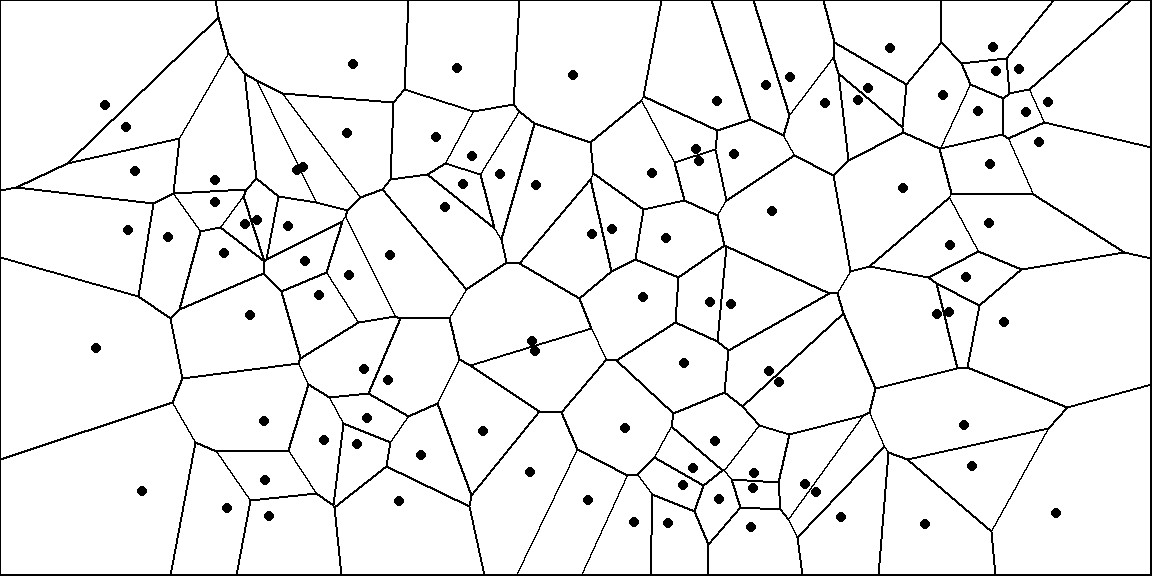
Voronoi Diagrams
A Voronoi diagram defines barriers around a set of points:

We can extend this to objects to generate paths that stay equidistant from objects.
Bushfire Planning
This calculates the distance to the nearest obstacle:
- Approximates the repulsive function for a potential field.
- Neighbours are either 4 point or 8 point connectivity.

We can calculate the grid like so:
- Label all empty cells as 0, and occupied cells as 1.
- Assume $i=1$
- For each cell neighbouring a cell with the value $i$, label it with $i+1$.
- Repeat until all cells have a non-zero value.
We can then compute paths by following the gradient around the map.
Higher numbers are more attractive cells.
Topological Maps
Topological maps record:
- Nodes - Representing areas in the world.
- Arcs - Representing adjacency and traversability between nodes.
By making a map into a graph, we can use graph searching algorithms to finds routes around a space.
Topological Map Types
Topological:
- Route based.
- Express space in terms of connections between landmarks.
- Orientation cues are egocentric.
Quantitative:
- Layout based.
- Independent of the robot pose.
Search
With grid based maps we can consider each cell as a node with $N4$ or $N8$ connectivity.
To find the way to a destination we will need to search the map for a route. To do this we can use the following search techniques:
- Naive searches:
- Depth-first Search
- Breadth-first Search
- Heuristic Searches:
- Dijkstra’s Shortest Path
-
Greedy Best-first Search
This is much faster than Dijkstra’s but is suboptimal and can be lured into local minima.
- A* Search
-
D* Search
This is a version of A* that keeps track of the search that led to a plan and only fixes the errors. This is faster than replanning from scratch.
- Wavefront Planning
Waypoints
As we find a route we should record waypoints, typically at the centre of each cell.
This is also known as local path planning. The goal is to avoid obstacles without the use of a map.
This is implemented as a subsumption behaviour, second to the main task.
Bug Algorithms
These are simple obstacle avoidance algorithms that assume:
- The robo has only local knowledge and the global goal.
- Robot modelled as a point operating on a plane.
- Sensor is tactlie (touch).
- Simple behaviours:
- Follow the wall
- Move in a straight line towards the goal
Success is guaranteed (where possible).
Bug 0
In this method it is assume we know that start and end points:
- Head towards the goal.
- If an obstacle is detected, follow the boundary (usually in a fixed direction) until you can head to the goal.
This can be foiled by certain obstacles.
Bug 1
To solve the issues in bug 0 we can remember where we have been.
- Follow along the obstacle to avoid it.
- Fully circle each encountered obstacle to be sure you know where the closest point is to the goal.
- Move to the point along the current obstacle boundary that is closest to the goal.
- Move towards the goal.
This can result in the following distances:
\[D\leq L_\text{Bug1}\leq D+1.5\sum_i P_i\]
where:
- $D$ - straight line distance from start to goal.
- $P_i$ - perimeter of the $i^\text{th}$ obstacle.
This method performs an exhaustive search to find the optimal leave point.
Bug 2
We can modify on the bug 1 algorithm:
-
Assume a straight path from start to the end goal.
Call this the $m$-line.
- Head to the goal on the $m$-line.
- If an obstacle is encountered, follow around the boundary until the $m$-line is encountered.
- Leave the obstacle and move towards the goal along the $m$-line.
This will result in the following distance:
\[D\leq L_\text{Bug2}\leq D+\frac 12\sum_i^n n_iP_i\]
where:
- $D$ - straight line distance from start to goal.
- $P_i$ - perimeter of the $i^\text{th}$ obstacle.
- $n_i$ - number of intersection points of the $i^\text{th}$ obstacle.
$L_\text{Bug2}$ can be arbitrarily longer than $L_\text{Bug2}$ if an obstacle has many intersecting points with the $m$-line.
This method performs an opportunistic approach. It is greedy and opts for the first promising approach found.
This is better for simple obstacles.
This is where we model the world as a 2D or 3D array. We can then store the probability that we are in any one location in this array.
Piecewise Constant Representation
Markov localisation utilised a probability distribution across all states:
- Represented as $\text{Bel}(x_t)$ for each $x_t$.
We can model this discretely as a histogram (bins):
The sum over all bins should be:
\[\sum x_t=1\]
We can then calculate like so:
- Start with a uniform distribution (if the location is unknown), or bounded Gaussian (if a location is known).
- The robot observes a feature:
- The robot now moves:
- We convolve out current distribution with our motion model.
- This translates the histogram and smooths peaks.
-
This is represented as:
\[\sum_{x_{t-1}}P(x_t\mid u_t,x_{t-1})Bel(x_{t-1})\]
-
The final distribution is the product of the observation model and resulting distribution with the shifted motion model:
\[Bel(x_t)=\eta P(z_t\mid x_t)\sum_{x_{t-1}}P(x_t\mid u_t,x_{t-1})Bel(x_{t-1})\]
$\eta$ is a normalisation factor that ensures $\sum x_t=1$.
Markov localisation is very computationally and memory intensive as all the bins have to be updated.
- Particle filters use sampling techniques to reduce the number of possible positions, and number of calculations.
We can describe the method like so:
-
Given a space, generate randomly, a set of particles that generate a hypothesis for where the robot.
Particles have a location and rotation (pose).
- Cull particles who’s observations don’t correlate with the current robot’s observations. These particles have low weight.
- For each particles that is culled, resample the space to find a location with greater likelihood.
A pseudo-code implementation of this is available at slide 33.
Using Ceiling Maps for Localisation
We can use ceiling lights to localise a robot by:
Kidnapping Problem
With our current approach for particles filters, we won’t be able to localise if there is an error, or the robot is manually moved. We can account for this by:
-
Randomly inserting a fixed number of samples with randomly chosen poses.
This corresponds to the assumption that the robot can be teleported at any point in time, to an arbitrary location.
We have seen a couple of types of maps in prior lectures:
this covers how to make these types of maps.
The General Mapping Problem
We can create a map from a run of:
- Controls (poses)
- Observations
Given the sensor data and poses, we want to calculate a map with the maximum likelihood given the data.
2D Volumetric Maps
This map assumes the world is a discrete set of cells:
- Each cell is either white (empty), or black (occupied).
Counting Model
You drive around, keeping track of where you are, and looking at each cell:
- You keep count of how many times you detect an obstacle in a cell.
- You increase the count each time you detect an object in it.
- You decrease the count for the cell each time you detect that it is clear.
By also counting how many times you have seen the cell (the count), you can estimate the probability that the cell is occupied.
Given that $M$ is a matrix of measurements and $C$ is a matrix of counts, we can calculate the probability that the cell is occupied like so:
\[P(m_{x,y})=\frac{M_{x,y}+C_{x,y}}{2C_{x,y}}\]
Binary Bayes Filters with Static State
Many problems can be addressed if we assume a binary, static state:
- The state doesn’t change during the observations.
- The state of an object is binary.
Given that the state doesn’t change, then maps can be estimated from:
\[p(m\mid z_{1:t},x_{1:t})=\prod_i p(m_i\mid z_{1:x},x_{1:t})\]
where the pose of each observation $z_{1:t}$ was $x_{1:t}$.
This gives us a binary Bayes filter for a static state.
Binary Random Variable
The area in the environment corresponding to a cell is modelled as:
- completely empty or occupied.
A cell is therefore a binary random variable.
Cell Independence
If we assume cell independence, the posterior is determined by the product of independent cell posteriors:
\[\prod_i p(m_i)\]
Log Odds
Odds are the ratio of the probability of an event $p(x)$ over the probability of its negated form $p(\neg x)$:
\[\text{odds}=\frac{p(x)}{p(\neg x)}=\frac{p(x)}{1-p(x)}\]
Logarithms are useful when odds are frequently multiplied or divided as:
\[\log ab=\log a +\log b\]
It is more efficient to add than multiply.
The log odds ratio is defined as so:
\[l(x)=\log\frac{p(x)}{1-p(x)}\]
we can then retrieve the probability from the log odds form, using the exponential function:
\[p(x)=1-\frac1{1+\exp l(x)}\]
The log odds model is given like so:
\[l(m_i\mid z_{i:t},x_{1:t})=\underbrace{l(m_i\mid z_t,x_t)}_\text{inverse sensor model}+\underbrace{l(m_i\mid z_{1:t-1},x_{1:t-1})}_\text{recursive term}-\underbrace{l(m_i)}_\text{prior}\]
There is a full example on how to derive this from slides 28-42.
Occupancy Mapping Update Rule
There is a simplified implementation for an update function using log odds at slide 48.

