Odometry & Wheel Encoders
Typical Motion Models
Typically there are two types of motion model:
- Odometry-based
- Used when systems are equipped with proprioceptive sensors such as wheel encoders.
- Velocity-based (Dead reckoning)
- Used based purely on velocities and time elapsed, using no sensors.
Classification of Sensors
Proprioceptive Sensors
Measure values internally, measuring direct feedback on the robot. This can include:
- Wheel Encoders
- Motor Load
Exteroceptive Sensors
Measure values from the environment. These can be:
- Ambient light sensors
- Radar
Passive Sensors
Measure energy from the environment, have no external effect. They can include:
- Accelerometers
- Thermometers
Active Sensors
Emit their own energy and measure the reaction. These include:
- IR emitters
- Sonar
Coping with Errors
In general odometry doesn’t hold up well over long distances:
- Range Error
- Integrated path length (distance) of the robots movement.
Sum of the wheel movements.
- Drift Error
- Difference in the error of the wheels leads to an error in the robot’s angular orientation.
- Turn Error
- Similar to range error, but for turns.
Difference of the wheel motions.
Over long periods of time, turn and drift errors far outweigh range errors.
Relative Odometry
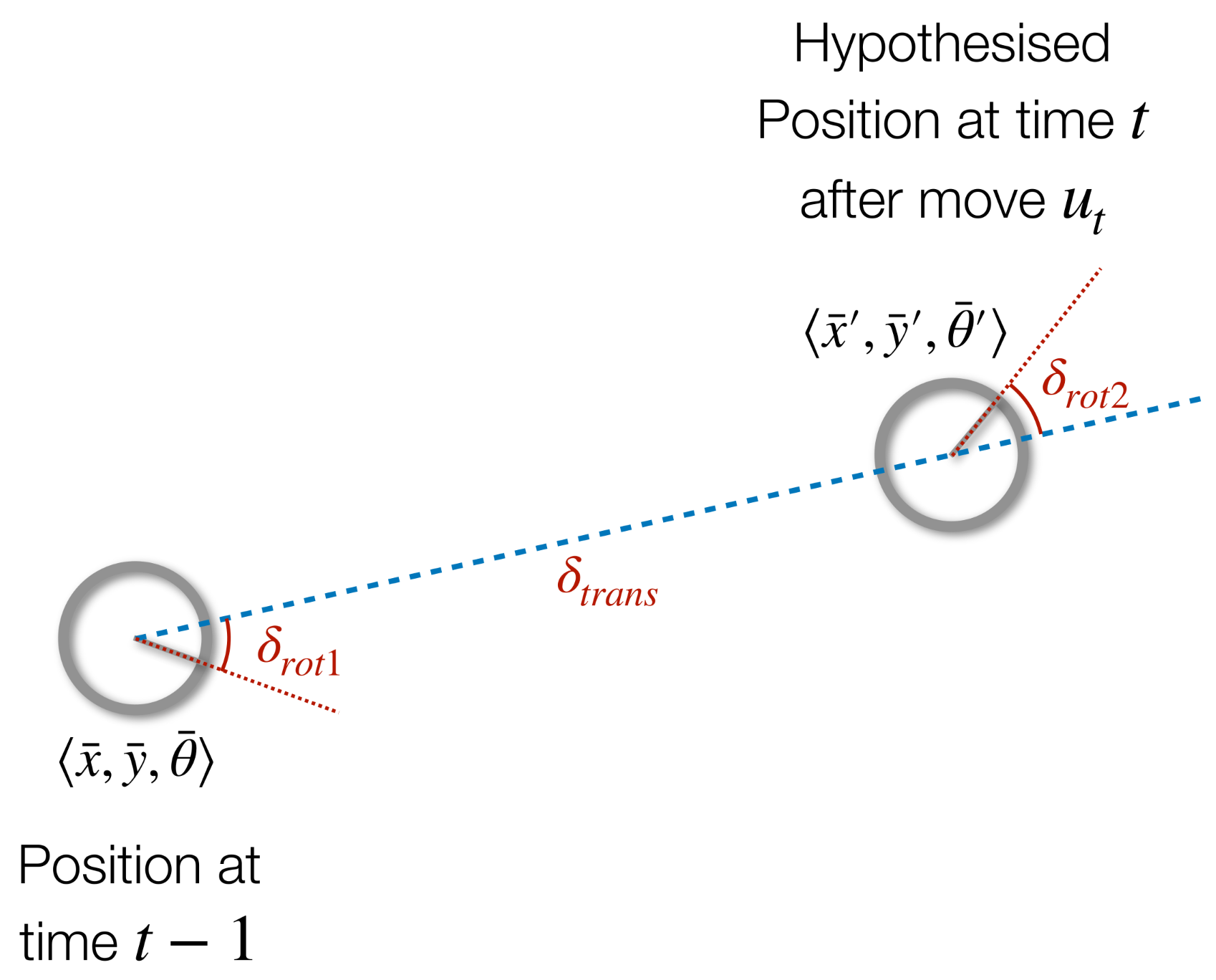
We can encode a position like so:
\[\langle x,y,\theta\rangle\]Where $x$ and $y$ are the Cartesian coordinates and $\theta$ is the direction the robot is facing:

We can write our believed position as $\langle \bar x,\bar y,\bar\theta\rangle$. This is opposed to the true location which is written as $\langle \hat x,\hat y,\hat\theta\rangle$
Odometry is the difference between two poses:
\[u=\langle\delta_\text{rot1},\delta_\text{trans},\delta_{rot2}\rangle\]where:
\[\begin{align} \delta_\text{rot1}&=\text{atan2} (y'-y,x'-x)-\theta\\ \delta_\text{trans}&=\sqrt{(x-x')^2+(y-y')^2}\\ \delta_\text{rot2}&=\theta'-\theta-\delta_\text{rot1} \end{align}\]$\text{atan2}$ is defined as so:
\[\text{atan2}(y,x) = \begin{cases} \arctan(\frac yx)&\text{if }x>0\\ \text{sign}(y)(\pi-\arctan(\lvert \frac yx\rvert))&\text{if }x<0\\ 0&\text{if }x=y=0\\ \text{sign}(y)\frac\pi2&\text{if }x=0,y\neq0 \end{cases}\]Odometry Model
What is the likelihood that $u_t$ took us from $\bar x_{t-1}$ to $\bar x_t$?
Where $\bar x_{t-1}$ and $x_t$ are our believed location before and after respectively.
We can determine the true odometry $\hat u_t$ via a model:
- We are trying to determine $p(\hat u_t\mid u_t)$ which can be solved by determining $p(x_t\mid u_t,x_{t-1})$, where:
- new location/state: $\text{pose}(x_t)$
- the motion/action: $\text{odometry}(u_t)$
- original location/state: $\text{pose}(x_{t-1})$
Model for Odometry with Noise
To calculate the true motion we should account for independent noise. We can do this using six coefficients $\alpha_1,\ldots,\alpha_6$. These can be calculated using sampling.
Noisy Initial Rotation
\[\hat\delta_\text{rot1} = \delta_\text{rot1}+\epsilon_{\alpha_1\lvert\delta_\text{rot1}\rvert+\alpha_2\lvert\delta_\text{trans}\rvert}\]Note that we take the absolute value using $\lvert x\rvert$. This doesn’t mean given that.
where:
- $\alpha_1$ - possibly due to error on the inital rotation.
- $\alpha_2$ - possibly due to forces on the robot as it moves forward.
Noisy Translational Error
\[\hat\delta_\text{trans}=\delta_\text{trans}+\epsilon_{\alpha_3\lvert\delta_\text{trans}\rvert+\alpha_4\lvert\delta_\text{rot1}+\delta_\text{rot2}\rvert}\]where:
- $\alpha_3$ - possibly due to error with the translation.
- $\alpha_4$ - initial and final rotation can result in a drift in position.
Noisy Final Rotation
\[\hat\delta_\text{rot2}=\delta_\text{rot2}+\epsilon_{\alpha_5\lvert\delta_\text{rot2}\rvert+\alpha_6\lvert\delta_\text{trans}\rvert}\]where:
- $\alpha_5$ - possibly due to error on the final rotation.
- $\alpha_6$ - possibly due to the resulting translational movement that may further rotate the robot.
Many models assume that the initial and final rotations have similar characteristics and assume $\alpha_5=\alpha_1$ and $\alpha_6=\alpha_2$.
Modelling $\epsilon$
-
We can use a Gaussian (normal distribution):
\[\epsilon_{\sigma^2}(x)=\frac1{\sqrt{2\pi\sigma^2}}e^{-\frac{x^2}{2\sigma^2}}\] -
We can use a triangular distribution as a fast approximation:
\[\epsilon_{\sigma^2}(x)=\begin{cases}0&\text{if }\lvert x\rvert>\sqrt{6\sigma^2}\\\frac{\sqrt{6\sigma^2}-\lvert x\rvert}{6\sigma^2}\end{cases}\]
The distributions have a zero-centred mean, and $b=\sigma=\text{standard deviation}$.